Kalman Filter Synchronization
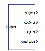
Single Phase Kalman Filter Synchronization component in Schematic Editor, which generates an output signal whose phase is related to the phase of an input signal and another signal with a 90 degree phase difference.
Description
The Kalman Filter Grid Synchronization algorithm is based on three main blocks. The first one is an observer, that contains the model of the grid and whose input is the error between the model output and the grid voltage. The single-phase grid is modeled as:
A state observer for this model can be defined as follows:
The second block contains the Kalman Filter algorithm, which finds the optimum gains for the observer to track the grid voltage at its output.
Finally, the third block is an algorithm that identifies the frequency, whose output is the reference to tune the observer model on the fundamental frequency (identified grid frequency). The base of the frequency identification algorithm, in state space, is given by:
This dynamic system works with error identification and grid frequency signal update equations, as detailed in [1] to generate the frequency signal that is used by the state observer.
Behavior and Features
The Kalman Filter Synchronization presents quick convergence and an accurate phase signal equivalence to the grid signal.
In the initial sampling steps the Kalman gain converges very quickly to optimum values, after which it is no longer needed to run the Kalman Filter algorithm. From this point, the synchronization algorithm behaves like a state observer with optimum gains.
Therefore, it is required to feed the input voltage at the first run of the synchronization algorithm to guarantee the correct convergence of filter gains. During the first three to five sampling steps the output signal can present undesirable peaks, so it is a good practice to wait for some samples to start using the synchronized signal.Although the identified frequency of the input signal is available as an output, it is an internal signal of the algorithm and should not be taken as an exact measurement of the input signal frequency.
Ports
- Vgrid (in)
- Sinusoidal input of the single-phase system from which the phase and frequency is
intended to be extracted.
- Supported types: real.
- Vector support: no.
- Sinusoidal input of the single-phase system from which the phase and frequency is
intended to be extracted.
- sin(wt) (out)
- Value of the trigonometric function ‘sin’ applied to the value of the phase of the
single-phase system.
- Supported types: real.
- Vector support: no.
- Value of the trigonometric function ‘sin’ applied to the value of the phase of the
single-phase system.
- cos(wt) (out)
- Value of the trigonometric function ‘cos’ applied to the value of the phase of the
single-phase system.
- Supported types: real.
- Vector support: no.
- Value of the trigonometric function ‘cos’ applied to the value of the phase of the
single-phase system.
- f[Hz] (out)
- Frequency (Hz) of the single-phase input system.
- Supported types: real.
- Vector support: no.
- Frequency (Hz) of the single-phase input system.
- Amplitude (out)
- Peak amplitude of the output signals,
.
- Supported types: real.
- Vector support: no.
- Peak amplitude of the output signals,
.
Properties
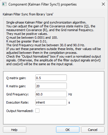
- Q matrix gain
-
Kalman Filter state covariance matrix gain.
-
- R matrix gain
- Kalman Filter measurement covariance matrix gain.
- Grid Frequency (Hz)
- Is the frequency value used to initialize the frequency identification algorithm.
- Output normalized
-
If checked, the output will be normalized. Otherwise the output signal will have the same amplitude as the input signal.
-
- Execution rate
- Type in the desired signal processing execution rate. This value must be compatible with other signal processing components of the same circuit: the value must be a multiple of the fastest execution rate in the circuit. There can be up to four different execution rates. To specify the execution rate, you can use either decimal (e.g. 0.001) or exponential values (e.g. 1e-3) in seconds. Alternatively, you can type in ‘inherit’ in which case the component will be assigned execution rate based on the execution rate of the components it is receiving input from.
References
[1] Cardoso, R.; de Camargo, R.F.; Pinheiro, H.; Gründling, H.A.: "Kalman filter based synchronisation methods", IET Generation, Transmission & Distribution, 2008, 2, (4), p. 542-555, DOI: 10.1049/iet-gtd:20070281IET Digital Library, https://ieeexplore.ieee.org/document/1712058