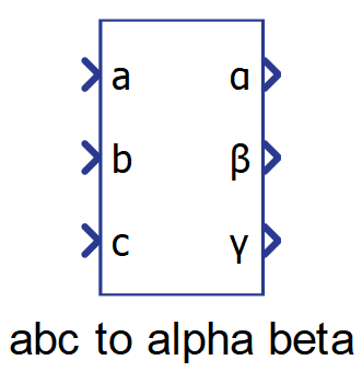
ABC to Alpha Beta
Description of the abc to alpha beta component in Schematic Editor, which performs an performs an ABC to αβγ transformation.
Description
This component performs the ABC to αβγ transformation, also known as Clarke's transformation. This transformation projects the three-phase quantities onto two stationary axes when the three-phase system is balanced. There are three modes for this transformation:
- Variant power - Clarke's original - The original transformation proposed by Edith Clarke. The γ axis is squashed which makes this output equal to the zero sequence obtained from the symmetrical components transformation. This transformation is power variant since the transformation matrix is not unitary.
- Variant power - uniform - Adaptation of Clarke's original transformation to keep all axes uniform. Since the γ axis is not squashed, this output is different from the zero sequence of the symmetrical components transformation. The transformation matrix is not unitary, thus the power is variant.
- Invariant power - Adaptation of Clarke's original transformation to keep all axis uniform while having a unitary transformation matrix. The power computation after this transformation is the same as the computation done before it. Since the γ axis is not squashed, this output is different from the zero sequence of the symmetrical components transformation.
ABC to alpha-beta-gamma Variant power - Clarke's original transformation matrix:
ABC to alpha-beta-gamma Variant power - uniform transformation matrix:
ABC to alpha-beta-gamma Invariant power transformation matrix:
The matrix computation is implemented with an optimized code as follows:
Where for Variant power - Clarke's original , and ;
for Variant power - uniform , and ;
and for Invariant power , and .
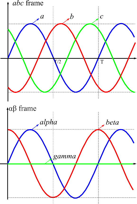
Figure 2 illustrates the transformation of a three-phase abc frame into an alpha beta frame using amplitude invariant transformation.
Ports
- a (in)
- Input a of the component, corresponding to the three-phase abc
system.
- Supported types: uint, int and real.
- Vector support: no.
- Input a of the component, corresponding to the three-phase abc
system.
- b (in)
- Input b of the component, corresponding to the three-phase abc
system.
- Supported types: uint, int and real.
- Vector support: no.
- Input b of the component, corresponding to the three-phase abc
system.
- c (in)
- Input c of the component, corresponding to the three-phase abc
system.
- Supported types: uint, int and real.
- Vector support: no.
- Input c of the component, corresponding to the three-phase abc
system.
- α (out)
- Output signal of the component related to the alpha signal of the alpha
beta gamma sequence frame.
- Supported types: real.
- Vector support: no.
- Output signal of the component related to the alpha signal of the alpha
beta gamma sequence frame.
- β (out)
- Output signal of the component related to the beta signal of the alpha
beta gamma sequence frame.
- Supported types: real.
- Vector support: no.
- Output signal of the component related to the beta signal of the alpha
beta gamma sequence frame.
- γ (out)
- Output signal of the component related to the gamma signal of the alpha
beta gamma sequence frame.
- Supported types: real.
- Vector support: no.
- Output signal of the component related to the gamma signal of the alpha
beta gamma sequence frame.
Properties
- Power transformation form
-
Allows choosing between the methods to perform the transformation. The methods available are:
-
Variant – Clarke's original: Use this method when you want the resulting alpha beta rotating frame to be amplitude invariant. That is, the amplitude of the original three-phase system will be preserved in the alpha beta stationary frame.
-
Variant – uniform: Use this method when the input ‘abc frame’ signal is a balanced system and you want the resulting alpha beta stationary frame to be amplitude invariant.
-
Invariant: Use this method when you want the resulting alpha beta stationary frame to be power invariant. That is, the power of the original three-phase system will be preserved in the alpha beta stationary frame.
-
-
- Execution rate
- Type in the desired signal processing execution rate. This value must be compatible with other signal processing components of the same circuit: the value must be a multiple of the fastest execution rate in the circuit. There can be up to four different execution rates. To specify the execution rate, you can use either decimal (e.g. 0.001) or exponential values (e.g. 1e-3) in seconds. Alternatively, you can type in ‘inherit’ in which case the component will be assigned execution rate based on the execution rate of the components it is receiving input from.