Capture
Description of the Capture functions of the Capture/Scope widget in HIL SCADA
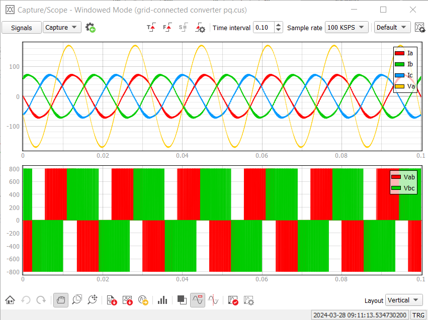
When the Capture/Scope Widget is in Capture mode (Figure 1), you can easily capture the desired signals directly from the connected HIL device or create custom Virtual signals. It also provides a means for a basic preview of the captured signals.
Captured signals can be saved to disk in various data formats.
The toolbar contains the basic capture parameters which you can set – sample rate and time interval.
Clicking  opens
the Signals window (Figure 2). This window contains a dynamic table where you can easily add (
opens
the Signals window (Figure 2). This window contains a dynamic table where you can easily add ( ) and remove
(
) and remove
( ) analog,
digital or Virtual
signals. In the first column, there is a combo box with all analog and digital
signals that exist in the loaded Model and all created Virtual signals that exist in the current
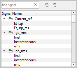
Panel. You can select a signal from the combo box or from the tree preview by clicking
) analog,
digital or Virtual
signals. In the first column, there is a combo box with all analog and digital
signals that exist in the loaded Model and all created Virtual signals that exist in the current
Panel. You can select a signal from the combo box or from the tree preview by clicking  (Figure 3). Double-clicking on a signal in the tree
selects that signal.
(Figure 3). Double-clicking on a signal in the tree
selects that signal.
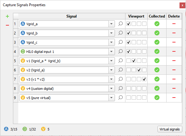
In the second column you can find check boxes that represent subplots. By checking them, you can select on which subplots the signal is going to be plotted. All subplots share the same x-axis zooming level.
The third column indicates if the signal is collected from the HIL device.
The last column contains an option for deleting the corresponding row from the table.
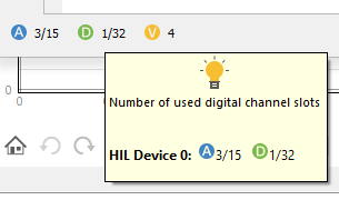
Below the signal table is a small legend that shows the number of used analog and digital signal slots combined for all HIL devices together with information how many Virtual signals are selected. Hovering the mouse over the legend brings up a small tool-tip (Figure 4) with more information about the used analog and digital slots for each used HIL device in the loaded Model.
Clicking ![]() opens the Capture Trigger Settings window (Figure 5). You also have the option to import previously saved
settings from the Scope tool with the Import signal settings from Scope button
(
opens the Capture Trigger Settings window (Figure 5). You also have the option to import previously saved
settings from the Scope tool with the Import signal settings from Scope button
(![]() ).
).
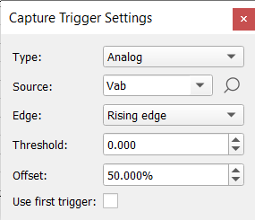
In this window, you can set the type of trigger to Analog, Digital, or User. For source, when the Analog or Digital trigger type is selected, you can choose from signals that were added previously in the Signals window using the combo box or the tree view, which is the same as the one in the Signals window. Edge of the trigger can be rising or falling. For threshold and offset you can type values with an accuracy of three decimal spaces. With the Use first Trigger checkbox you can define a trigger behaviour when an offset is set (False (uncehcked)- any trigger occurrence will be ignored until the offset is satisfied, True (checked) - the first trigger occurrence will be used despite the desired offset).
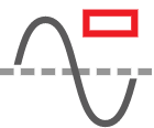
- Execute the Force trigger and retrieve data without offset,
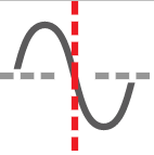
- Enter the Enable trigger mode to start data acquisition and then execute the Force trigger to retrieve data with the desired offset.
Besides the functionalities shown above, you can also use the following ones:
 Enable trigger - enables the trigger in the capture mode.
 Force trigger - forces the trigger functionality in the capture mode.
 Stop capture process - stops Capture process.Note: All data collected by HIL device before Capture process was stopped will be downloaded and displayed.
In addition to the basic options (Capture and scope mutual functions), Capture mode has these additional options:
 Undo action - undo
an action on the Capture widget (pan, zoom, and any X and Y
axis range changes).
Undo action - undo
an action on the Capture widget (pan, zoom, and any X and Y
axis range changes). Redo action - redo
an action on the Capture widget (pan, zoom, and any X and Y
axis range changes).
Redo action - redo
an action on the Capture widget (pan, zoom, and any X and Y
axis range changes). Pan move - pan axes.
 Rectangle zoom - zoom with an arbitrary rectangle selector.
 Constrained zoom - zoom using a constrained vertical or horizontal rectangle
selector.
Constrained zoom - zoom using a constrained vertical or horizontal rectangle
selector. Zoom to fit - automatically adjust the plot view so all data points are visible within the window
 Zoom to user range - automatically adjust the plot view according to the User specified zoom
 User Range settings - Opens the dialog for editing User specified zoom
 Save signals to file - opens Signal Data Saving, which allows you to save all or selected signals to various data formats.Note: Currently supported formats are: CSV, HDF5, NI TDMS, MAT, MDF4, COMTRADE CFF.
 Export to PNG image - takes a screenshot of the Capture widget's
plots and saves it as a .PNG image.
Export to PNG image - takes a screenshot of the Capture widget's
plots and saves it as a .PNG image. Export captured signals to Signal Analyzer tool - opens the Signal Analyzer tool and loads the currently captured
data.
Export captured signals to Signal Analyzer tool - opens the Signal Analyzer tool and loads the currently captured
data. FFT analysis - opens the FFT Analysis window and applies FFT to the currently captured data.
-
 Invert background color - inverts the background plot surface colors.
 -
 Show/hide legend - shows or hides the legend with signal names.
 -
 Under the mouse action - when enabled, this feature displays the x-value and corresponding signal values at the mouse position, but only when the cursor is hovering over a valid data point.
 -
 Trigger marker - toggles the trigger marker line on or off.
  Signals
properties - opens the Signal Properties, which
allows you to set the properties of the signals.
Signals
properties - opens the Signal Properties, which
allows you to set the properties of the signals.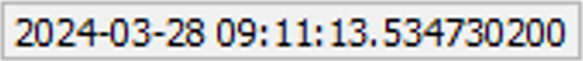 Trigger time indicator - Absolute UTC time when
trigger occurred. In case the Trigger time is not available, the
Trigger time indicator - Absolute UTC time when
trigger occurred. In case the Trigger time is not available, the  indicator will be shown. If
Trigger time is available, the UTC time and Timestamp
value can be copied by right-clicking on the Trigger time
indicator and selecting the corresponding option in the context menu (Figure 6).Note: Trigger time indicator information may not be available if the used HIL devices are not time synchronized or if Virtual HIL is used.
indicator will be shown. If
Trigger time is available, the UTC time and Timestamp
value can be copied by right-clicking on the Trigger time
indicator and selecting the corresponding option in the context menu (Figure 6).Note: Trigger time indicator information may not be available if the used HIL devices are not time synchronized or if Virtual HIL is used.Figure 6. Trigger time indicator context menu 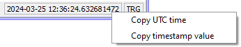
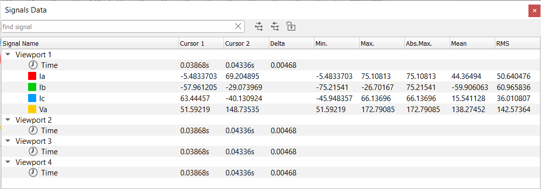
Signal data pane (Figure 7) enables you to measure the signals values at specified locations. Values that can be measured are:
- Positions of cursors 1 and 2
- Delta value
- Minimum (Min.), maximum (Max.), and absolute maximum (Abs. Max.)
- Mean and RMS values
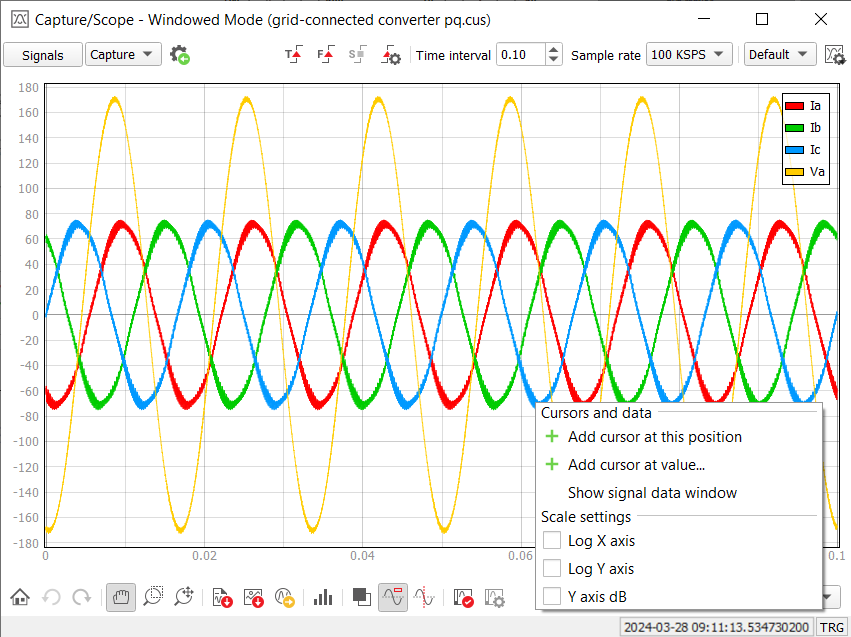
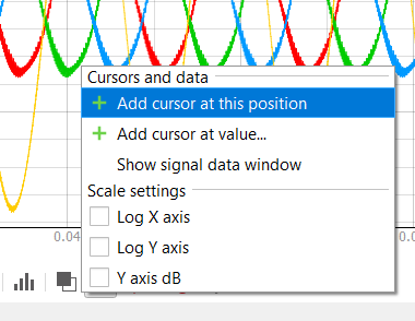
Right click context menu
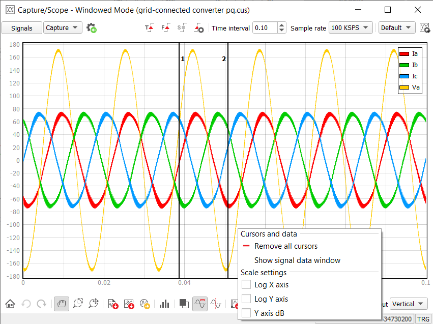
By right clicking on a plot, you can bring up the context menu which holds various actions that you can perform on the plot. Some allow you to change the currently displayed scales, while others allow you to add and remove cursors which are used for detailed signal analysis.
-
Log X axis - by clicking on this action within the context menu, you will toggle between linear and log scale of the X axis.Note: This action can only be performed after Forcing the Capture Trigger, since that's when the X axis values start from zero. In this case, the first data point will be omitted when toggled on. In any other case where X axis values contain negative values, an information dialog will be shown and the scale will remain linear.
- Log Y axis - by clicking on this action within the context menu, you will toggle
between linear and log scale of the Y axis. Note: This action can only be performed if the signals contain no non-positive values. If they do contain non-positive values, an information dialog will be shown and the scale will remain linear.
- Y axis dB - by clicking on this action within the context menu, you will toggle
between linear and dB scale of the Y axis. This action performs logarithmic scaling of
the signal values, with an additional multiplication of values by a factor of
20.Note: Just like normal log scaling of the Y axis, the same conditions must be met (no non-positive values can be present).
You can place cursors by right-clicking the menu inside the plot surface (Figure 9).
There is a maximum of two cursors that can be placed.
Once the cursor is placed it can be moved by left-clicking it and holding it.
A specific cursor can be removed by right-clicking it and choosing the “Remove cursor” option. If both cursors are placed, right-clicking the plot surface will give you an option to “Remove cursors” which, if selected, will remove both measurement cursors. (Figure 10)
If the Signal measurements window is closed, you can reopen it by choosing the Show Signal Data Window from the right click menu. (Figure 10)