Discrete Transfer Function
Description of the Discrete Transfer Function component in Schematic Editor, which represents a mathematical function which theoretically represents the system output for each possible input.
Component Icon
Description
The discrete transfer function of a system is a discrete representation of the continuous system in the s-domain discretized according to the sampling time Ts
The output H(z) of Discrete Transfer Function is calculated using following formula:
Where m+1 and n+1 are the number of numerator and denominator coefficients.Initial value of states of the transfer function are set to zero.
For example, if numerator is [1] and denominator is [1, -1], the transfer function will be:
- Bilinear,
- Euler,
- Backward differencing, and
- Zero-order hold.
Discretization methods
-
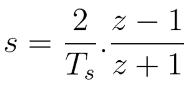
This method for converting a continuous system into a discrete system is called Bilinear, or Tustin transformation. It maps the left-hand complex plan in the s-domain into the unit circle in the z-domain. That is, for every stable point in the continuous system, the bilinear transformation will return a stable point in the discrete system.
This method relates the s-domain transfer function to the z-domain transfer function using the following approximation:
-
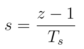
Euler discretization method, or forward discretization method uses the knowledge of the current signal, the time step, and the derivative of the signal, and approximates the slope between the current and next signal.
This is the simplest and probably least accurate method for discretizing a system and it is possible that a stable continuous-time system is mapped into an unstable discrete-time system.
This method relates the s-domain transfer function to the z-domain transfer function using the following approximation:
-
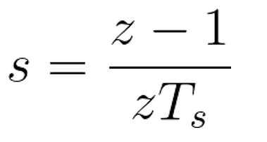
The backward Euler method is similar to the forward Euler approach except that it uses the next point as the point for calculating the derivative.
This method relates the s-domain transfer function to the z-domain transfer function using the following approximation:
-
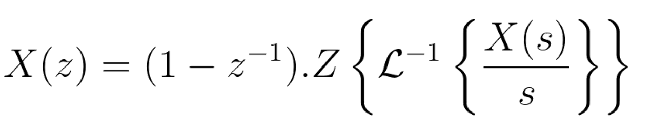
The zero-order hold method takes into account the discretization delay of a continuous system. This method of discretization relates the s-domain system and the z-domain system by the following approximation:
Ports
- Input (in)
- Original input signal.
- Supported types: uint, int, real.
- Vector support: yes.
- Original input signal.
- Output (out)
- Filtered signal.
- Supported types: uint, int, real, and inherit.
- o Output type is set from component’s parameter Signal out type or inherited from signal processing circuit.
- Vector support: yes
- Vector length is inherited from the input signal.
- Supported types: uint, int, real, and inherit.
- Filtered signal.
Properties
![]()
![]()
- Coefficients domain
- Choose the domain in which the transfer function will be declared. This property defines if the coefficients declared in the Numerator and Denominator properties are defined in the s-domain or in the z-domain. Available values for this property are Z-domain, or S-domain.
- Numerator
- Type in the coefficients of the numerator of the transfer function. It is declared as a python list in descending powers of ‘s’ or ‘z’.
- Denominator
- Type in the coefficients of the denominator of the transfer function. It is declared as a python list in descending powers of ‘s’ or ‘z’ and must have a higher order than the numerator.
- Signal out type
- Choose the type of the output signal of the component. This property can be set to “real”, “int”, “uint”, or “inherit”.
- Discretization method
-
Choose the discretization method. This property is shown only when Coefficients domain property is set as “s-domain” and it defines the discretization method for the continuous-time transfer function defined by the numerator and denominator of the component.
Available methods are: zero-order hold, Forward Euler, Backward Euler, and Bilinear (or Tustin).
-
- Execution rate
- Type in the desired signal processing execution rate. This value must be compatible with other signal processing components of the same circuit: the value must be a multiple of the fastest execution rate in the circuit. There can be up to four different execution rates. To specify the execution rate, you can use either decimal (e.g. 0.001) or exponential values (e.g. 1e-3) in seconds. Alternatively, you can type in ‘inherit’ in which case the component will be assigned execution rate based on the execution rate of the components it is receiving input from.