Home
Typhoon HIL Software Manual
Schematic Editor Component Libraries
Detailed functionality and use of the pre-built Component Libraries in Schematic Editor
Component library
This section describes the general properties of the component library in Schematic Editor, and provides a list of main types of components available in it.
Signal processing components
This section describes the general properties of all signal processing components in the Typhoon HIL Schematic Editor core library.
Signal Processing Sources
Summary of the Source components available through the Signal Processing category of the Schematic Editor core library.
Sinusoidal Source
Description of the Sinusoidal Source component in Schematic editor, which outputs a sinusoidal waveform

Typhoon HIL Software Manual
- Introduction
  Overview of the categories covered in the Typhoon HIL Software Manual
- System Requirements
  Guidelines for the hardware and/or software environment necessary to run Typhoon HIL Control Center, for both PC and Test Server/Virtual Machine-based setups.
- Typhoon HIL Quick Start Guide
- Typhoon HIL Toolboxes
  List of the Toolbox Packages available in the Typhoon HIL software suite
- Connecting to your HIL device
  Guidelines on how to connect to a HIL device using either USB or Ethernet ports.
- Device Manager
  Device Manager is used to create, manipulate, and activate HIL device setups.
- Typhoon HIL Control Center
  This section provides a general description of Typhoon HIL Control Center and lists the main software components accessible from it, as well as additional software tools which can be invoked from its interface.
- Example Explorer
  General Description of the Typhoon HIL Control Center Example Explorer.
- Signal Access Management
  This feature allows you to change the visibility of signals in Schematic Editor and HIL SCADA
- Schematic Editor
  Introduction to the Schematic Editor tool in Typhoon HIL Control Center
- Schematic Editor Component Libraries
  Detailed functionality and use of the pre-built Component Libraries in Schematic Editor
  - Modeling principles
    This section describes modeling principles used in Typhoon HIL's software.
  - Model partitioning
    This section describes the general motivation and gives some practical guidelines for model partitioning.
  - Component library
    This section describes the general properties of the component library in Schematic Editor, and provides a list of main types of components available in it.
    - Circuit breakers
      This section describes the general properties of all circuit breaker components in Typhoon HIL Schematic Editor. There are currently 2 different circuit breaker components in Schematic Editor.
    - Communication
      Summary of the Communication components available in Schematic Editor.
    - Contactors
      This section describes the general properties of all contactor components in Typhoon HIL's Schematic Editor. There are currently 2 different contactor components in Schematic Editor.
    - Converters
      This section provided a general description of converters in Schematic Editor, including converter control options, thermal model, variable delay, and the Measurements tab.
    - Converters - extras
      This section describes additional components related to converter modeling.
    - HIL Interfaces
      This section describes the HIL Interface components in Typhoon HIL Schematic Editor.
    - Machines
      This section describes the concepts used in the modeling and implementation of electrical machine components in Typhoon HIL Schematic Editor. There are currently 26 different machine components.
    - Measurements
      This section describes measurement components in Schematic Editor, including voltage and current measurements and RMS measurements.
    - Microgrid
      This section describes the Microgrid library category in Typhoon HIL Schematic Editor.
    - Circuit partitioning components
      This section describes the general properties of circuit properties components in Typhoon HIL's Schematic Editor, such as core couplings, device couplings, core markers, device markers, etc.
    - PHIL Interfaces
      This section describes the general properties of Power Hardware-In-the-Loop (PHIL) interface components.
    - Passive components
      This section describes passive components, including linear passive components, nonlinear passive components and variable passive components.
    - Port components
      Description of the collection of Port components in Schematic Editor, which are used to connect internal subsystem elements to the outside schematic.
    - Signal processing components
      This section describes the general properties of all signal processing components in the Typhoon HIL Schematic Editor core library.
      - Discrete
        This sub-category contains twelve discrete components: Accumulator, Integrator, Unit Delay, Delay, Transport Delay, Rate Limiter, Differentiator, FIR Filter, Discrete Transfer Function, Discrete State Space, Hysteresis Function, and Low Pass Filter.
      - Extras
        Summary of the Extra components in Schematic Editor
      - Functions and Tables
        Summary of the Functions and Tables components available in Schematic Editor.
      - Logical
        Summary of the Logical components available in Schematic Editor.
      - Math operations
        Summary of the Math Operations components available in Schematic Editor.
      - Power Measurements
        Summary of the Power Measurements components available in Schematic Editor.
      - Power Systems
        Summary of the Power Systems components available in Schematic Editor.
      - Sinks
        Summary of the Sinks components available in Schematic Editor.
      - Signal Processing Sources
        Summary of the Source components available through the Signal Processing category of the Schematic Editor core library.
        Analog Input
        Description of the Analog Input source component in Schematic editor, which outputs a value from a selected analog input.
        Clock
        Description of the Clock component in Schematic editor, which outputs the current simulation time in seconds.
        Constant
        Description of the Constant component in Schematic editor, which outputs a constant signal.
        Digital Input
        Description of the Digital Input source component in Schematic editor, which outputs a value from a selected digital input.
        Dynamic Table
        Description of the Dynamic Table component in Schematic editor, which outputs and repeats a custom value sequence imported from a file.
        Ramp
        Description of the Ramp component in Schematic Editor, which outputs a constantly increasing or decreasing signal.
        Repeating Sequence Discrete
        Description of the Repeating Sequence Discrete component in Schematic editor, which outputs and repeats a custom value sequence.
        SCADA Input
        Description of the SCADA Input component functionality in Schematic Editor
        Signal Picker Source
        Description of the Signal Picker Source component in Schematic Editor, which outputs a selected signal from the model.
        Sinusoidal Source
        Description of the Sinusoidal Source component in Schematic editor, which outputs a sinusoidal waveform
        Square Wave Source
        Description of the Square Wave Source component in Schematic editor, which outputs a Square waveform
        Step
        Description of the Step component in Schematic editor, which outputs a step function between two levels at a specified time.
        Triangular Wave Source
        Description of the Triangular Wave Source component in Schematic editor, which outputs a triangular waveform.
      - System
        Summary of the System signal processing components available in Schematic Editor.
    - Interface components
      This section describes the general properties of all interface components in Typhoon HIL's Schematic Editor, such as voltage and current measurements, signal-controlled sources, contactors, etc. There are currently 4 different interface components in Schematic Editor.
    - Sources
      This section describes source components in Schematic Editor, including independent sources, controlled sources, externally controlled sources, signal controlled sources, batteries, photovoltaic panels, constant power loads/sources, and engine-generator sources.
    - System
      This section describes additional components in the System library in Schematic Editor
    - Test Suite
      This section describes the Test Suite components of Typhoon HIL's built in Schematic Editor Library, which currently includes the grid simulator, DC measurements, anti-islanding container, and grid fault components.
    - Transformers
      This section describes the general properties of all transformer components in Typhoon HIL's Schematic Editor, such as an ideal transformer, a single-phase three winding transformer, a three-phase four winding transformer, etc. There are currently 9 different transformer components in Schematic Editor.
    - Transmission lines
      This section describes the general properties of all transmission line components in Typhoon HIL's Schematic Editor. There are currently 3 different transmission line components in Schematic Editor.
    - Component additional information
      This section describes the general properties of several components in Typhoon HIL's Schematic Editor whose feature set and capabilities require separate sections.
  - References
    This section describes references
- Third-party integrations
  This section provides an overview of the key third party integrations within Typhoon HIL's toolchain.
- HIL SCADA
  Description of the HIL SCADA tool in Typhoon HIL Control Center
- Waveform Generator
  This section describes the waveform generator tool in Typhoon HIL Control Center.
- Test and Calibration Tool
  Description of the Test and Calibration tool in Typhoon HIL Control Center
- TyphoonTest IDE
  This section describes TyphoonTest IDE
- Signal Analyzer
  This section describes the Signal Analyzer tool.
- Lookup table extraction tool
  Description of the Typhoon HIL Control Center tool for extracting characteristics (lookup tables) from datasheet graphs and charts into a format that can be imported by non-linear models.
- Package Manager
  Description of the Typhoon HIL Control Center tool for creating and managing Typhoon packages that contain Schematic examples, Schematic and widget libraries, documentation etc.
- Usage Logging
  This section briefly describes Typhoon HIL software logging feature.
- Python Interpreters
  Overview of how you can use Typhoon HIL Python Interpreters to further customize your test files.

Sinusoidal Source

Description of the Sinusoidal Source component in Schematic editor, which outputs a sinusoidal waveform

Component icon

Figure 1. Sinusoidal source icon

Description

The Sinusoidal source component outputs a sinusoidal waveform.

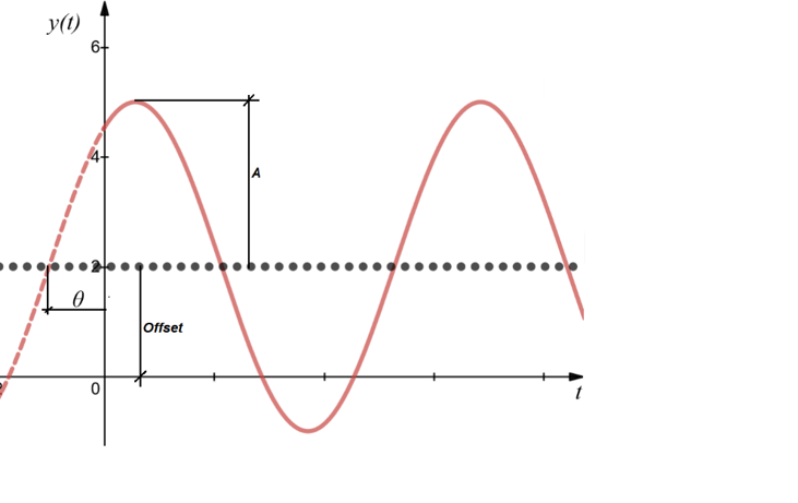
Sinusoidal source can be represented with a function

y(t) = Offset + A . sin(2.π.f + θ)

where:

Offset - is the DC offset value
A - is the sinusoidal waveform amplitude
f - is the frequency
θ - is the displacement angle for the sinusoidal waveform

An example of a sine waveform generated by this component is depicted below.

Figure 2. Example of a sinusoidal waveform produced by sinusoidal source component

Ports

Output (out)
- Sinusoidal waveform.
  - Supported types: real.
  - Vector support: yes.
    - The vector length is calculated from the property values. If the property is defined as a vector, the output will be a vector of the same length.

Properties

Amplitude
- Type in the peak value of the sinusoidal waveform. This property can be set as a scalar or a vector.

DC offset
- Type in the DC offset value to be added to the sinusoidal waveform. This property can be set as a scalar or a vector.

Frequency
- Type in the frequency value, in hertz, of the sinusoidal waveform. This property can be set as a scalar or a vector.

Phase
- Type in the value of the phase, in degrees, with which the sinusoidal waveform will be delayed in reference to the simulation start time. This property can be set as a scalar or a vector.

Execution rate
- Type in the desired signal processing execution rate. This value must be compatible with other signal processing components of the same circuit: the value must be a multiple of the fastest execution rate in the circuit. There can be up to four different execution rates, but they must all be multiple of the basic simulation timestep. To specify the execution rate, you can use either decimal (e.g. 0.001) or exponential values (e.g. 1e-3) in seconds. Alternatively, you can type in ‘inherit’ in which case the component will be assigned execution rate based on the execution rate of the components it is receiving input from.

Tunable
- Enables run-time tuning of the selected component. This will allow you to change values for frequency, DC offset, amplitude, and phase during simulation without the need to recompile the model. Tunable properties are available in HIL SCADA in Model Explorer.
- Phase can be tuned only before the start of the simulation.