Transformers
This section describes the general properties of all transformer components in Typhoon HIL's Schematic Editor, such as an ideal transformer, a single-phase three winding transformer, a three-phase four winding transformer, etc.
Core model
Transformer core modeling is available for all transformers in the library. A transformer core model can be selected by the Core model combo box. The list bellow describes mask properties and the primary side of the transformer for all available core models. Core model can be set to one of the following values:
- Linear
- The core is modeled as a linear magnetizing inductance on the primary side of the transformer
Figure 1. Primary side of a transformer with Core model set to Linear 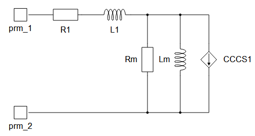
-
Non-Linear / Hysteresis
- The core saturation is modeled as a nonlinear magnetizing inductance on the primary side of the transformer. Some transformers can also model the hysteresis of the core.
Figure 2. Primary side of a transformer with Core model set to Non-Linear or Hysteresis 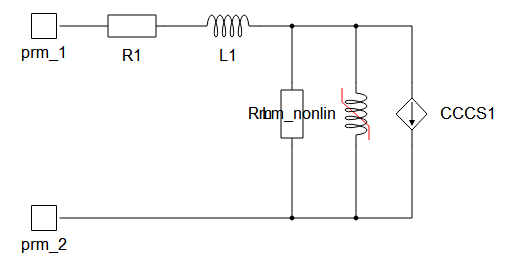
- Lm/Rm neglected
- When selected, the core magnetizing inductance and resistance will be neglected
Figure 3. Primary side of a transformer with Core model set to Lm/Rm neglected 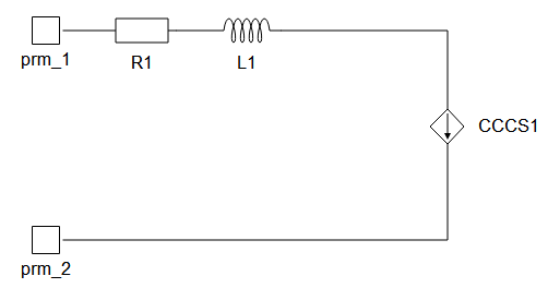
Hysteresis effects
Simulating hysteresis effects requires signal processing implementation. Therefore, an execution rate for hysteresis simulation must be specified. To capture this effect for an arbitrary dynamic signal, its period should be at least 20 times faster than the execution rate of hysteresis sampling, defined in Execution rate. Hysteresis is further defined through three lists/arrays which have different labels depending on the type of transformer or nonlinear inductor as shown in Figure 4.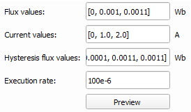
To properly define hysteresis, the data value for both Flux values and Hysteresis flux values must be specified for the zero current data-point, which means that the first value of Current values and Flux values lists/arrays must be 0, and that the first value of the Hysteresis flux values list/array must be the remanent flux value. Secondly, all three of these properties must have the same number of elements and all three must be monotonically non-decreasing lists/arrays. Hysteresis flux values must have at least one element that is higher in value than the corresponding element in the Flux values list, followed by at least one element that has the same value as the corresponding element in Flux values. The first common element for Hysteresis flux values and Flux values is defined as the Hysteresis upper curve threshold.
Figure 5 demonstrates an example of properly defined parameter values using the settings below.
Flux values [Wb]: [0, 0.004, 0.008, 0.011, 0.013, 0.014, 0.0145, 0.015]
Current values [A]: [0, 1, 2, 3, 4, 5, 6, 7]
Hysteresis flux values [Wb]: [0.004, 0.007, 0.01, 0.012, 0.0135, 0.0141, 0.0145, 0.015]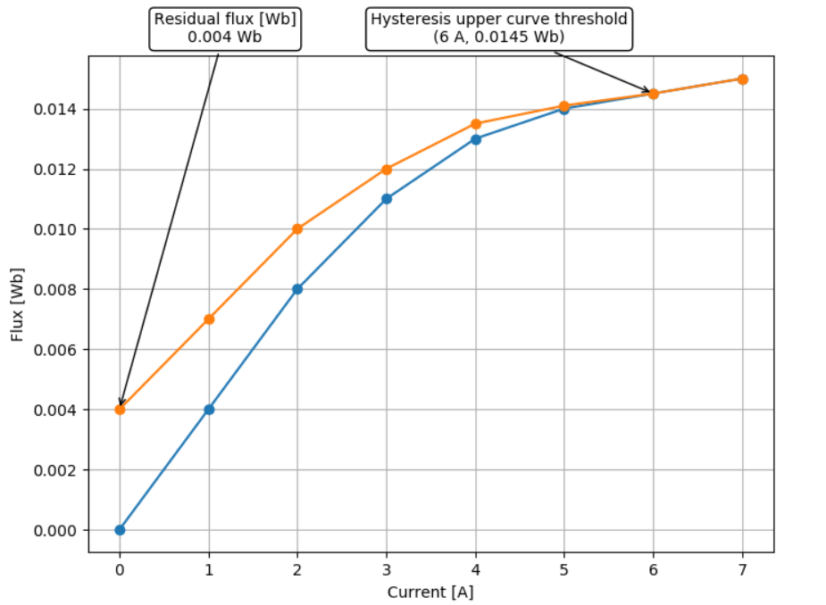
Clicking the Preview button will validate the hysteresis parameters, but only if they are defined directly in the respective property fields and not if they are defined through the namespace. After validation, the Hysteresis curve will be extended, showing the expected simulation hysteresis curve as shown in Figure 6.
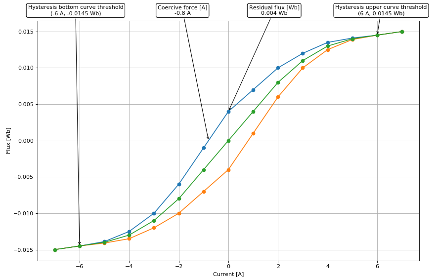
When the simulated flux value surpasses the Hysteresis upper curve threshold, the upper curve becomes the trajectory for the flux-current set-points and stays that way until the next trigger event. When the simulated flux value falls bellow the Hysteresis bottom curve threshold, the bottom curve becomes the trajectory for the flux-current set-points and stays that way until the next trigger event. When the simulation is first started, the original curve is a reference, until the next trigger event. A way to disable hysteresis and return the reference curve to the original magnetization curve during runtime, is to set the scada input named demagnetize_scada_in to 1. To re-enable the hysteresis upper and bottom curve, set the scada input demagnetize_scada_in to 0. Flux demagnetization to the reference curve is not supported in TyphoonSim yet.
The current version of Schematic Editor offers a selection of the following types of transformer components:
- Single Phase Four Winding Transformer
- Single Phase Multi-Winding Transformer
- Single Phase Three Winding Transformer
- Single Phase Two Winding Ideal Transformer
- Single Phase Two Winding Ideal Transformer With Variable Transfer Ratio
- Single Phase Two Winding Transformer
- Single Phase Two Winding Variable Ratio Transformer
- Three Phase Four Winding Transformer
- Three Phase Three Winding Transformer
- Three Phase Two Winding Phase-shifting Transformer
- Three Phase Two Winding Transformer
- Three Phase Two Winding Variable Ratio Transformer
Additional information on calculation of equivalent circuit parameter values is contained in a separate section.