UltraCore
Description of the UltraCore solver, which allows for real-time simulation of converter components using timestep equal to the period of the HIL device clock (down to 3.5 ns).
UltraCore introduction
UltraCore is a specialized hardware resource, present in some HIL device configurations (see Device Configuration Table). UltraCores are used in order to simulate the converter components that are located in the Enhanced Resolution converters sub-category of the Converters library category. At the moment, converter components in this category are:
UltraCore consists of two parts:
- the UltraCore execution unit
- the electrical circuit interface
The signals measured in the circuit interface are used as inputs to the UltraCore. The UltraCore execution unit then calculates the model outputs and feeds them to the sources in the circuit interface.
UltraCore execution unit
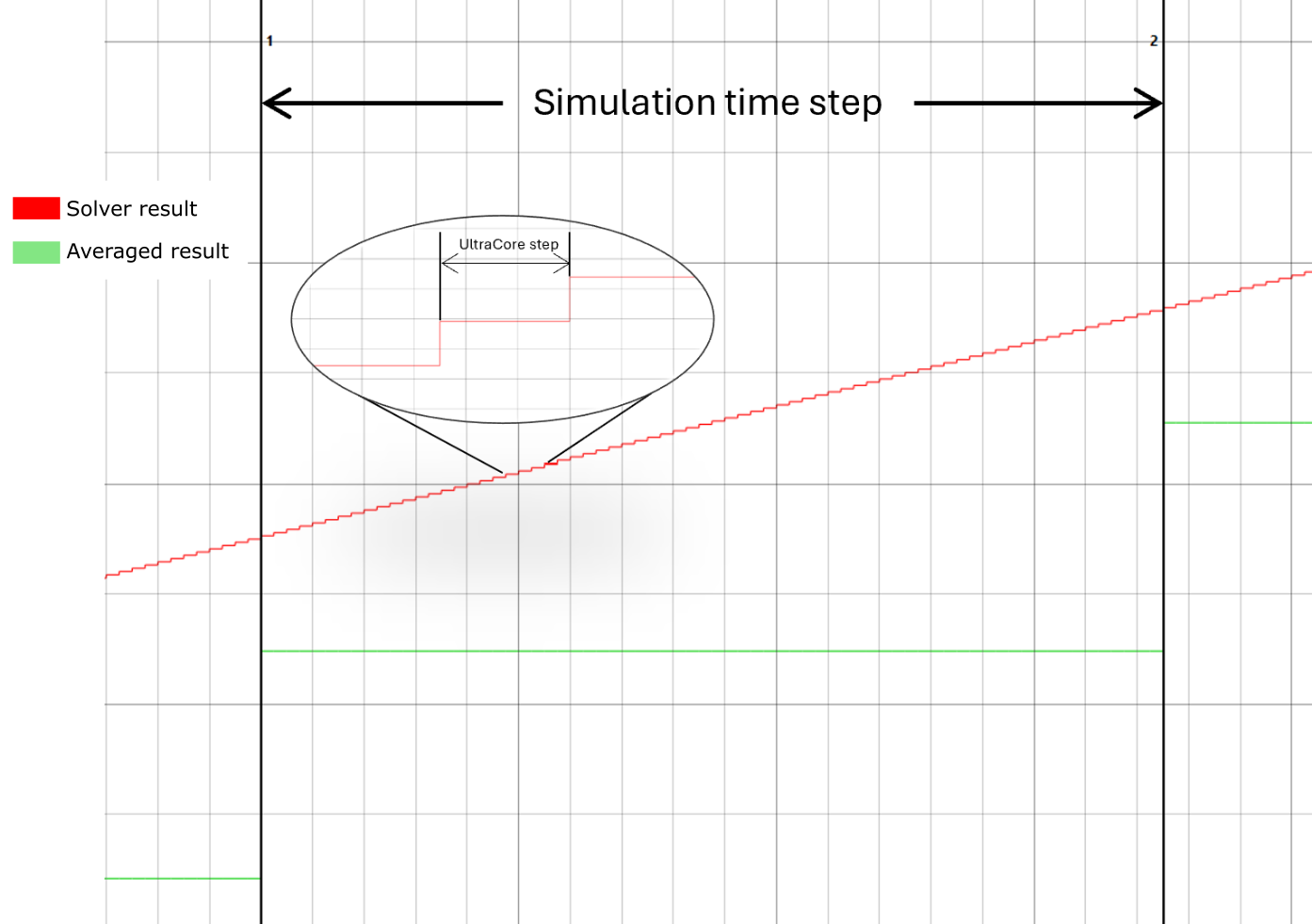
UltraCore offers the ability to simulate the dynamics of fast-switching converter topologies with enhanced time resolution. It does so by executing part of the model using very small timesteps. UltraCore timesteps are fixed, in the sense that they are independent from the simulation step used for the rest of the model (configured in Table 2). The UltraCore step used for the critical model variables is equal to the period of a HIL device clock: 3.5 ns for HIL404, HIL506, and HIL606; 4.5 ns for HIL101; and 6.25 ns for HIL602+, and HIL604. Critical model variables are the ones that determine the state of the switches by means of zero-crossing events, usually the diode currents.
- Output sources: Signals that are injected into the circuit in order to enable the solver to interact with the rest of the model (see Electrical circuit interface).
- Measurement signals: Analog signals that are calculated by the solver (inductors' currents, capacitors' voltages, etc.). These are available in the analog signals list.
<analog_signal_name>_cmp_out- They are updated at the end of every UltraCore step (every HIL device clock), thus reducing the loopback latency and improving the timing precision of the comparator signal edge.
- If these signals are used to drive a digital output of the HIL device, this output will be updated at UltraCore step rate, unlike the analog output signals that can only be updated at simulation step.
Electrical circuit interface
The UltraCore is an independent module on the FPGA. In Schematic Editor, it is instantiated as a converter block (see Converters). The converter component is configured like any other converter component and it invokes the solver automatically. No additional solver-specific configuration is needed.
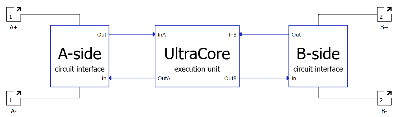
In order to interact with the rest of the model, measurements are used as an electrical input, while controlled sources are used as solver outputs, as shown in Figure 2. The electrical circuit interface depends on the topology that is being simulated using the UltraCore. In some cases measurements are voltage measurements and sources are current sources, while in other cases it is the opposite. Interface specifics for the topology that is being simulated is described in the documentation of that converter topology. The electrical circuit interface should be taken into consideration when using converters that are based upon the UltraCore, in order to avoid potential Topological Conflicts. Electrical circuit interface subcircuits (A-side and B-side) are electrically connected, meaning that the input and the output of the converter topology are placed into the same SPC.
Backward incompatibility resolution
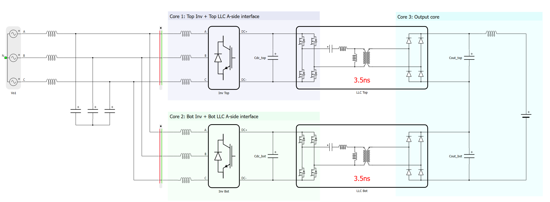
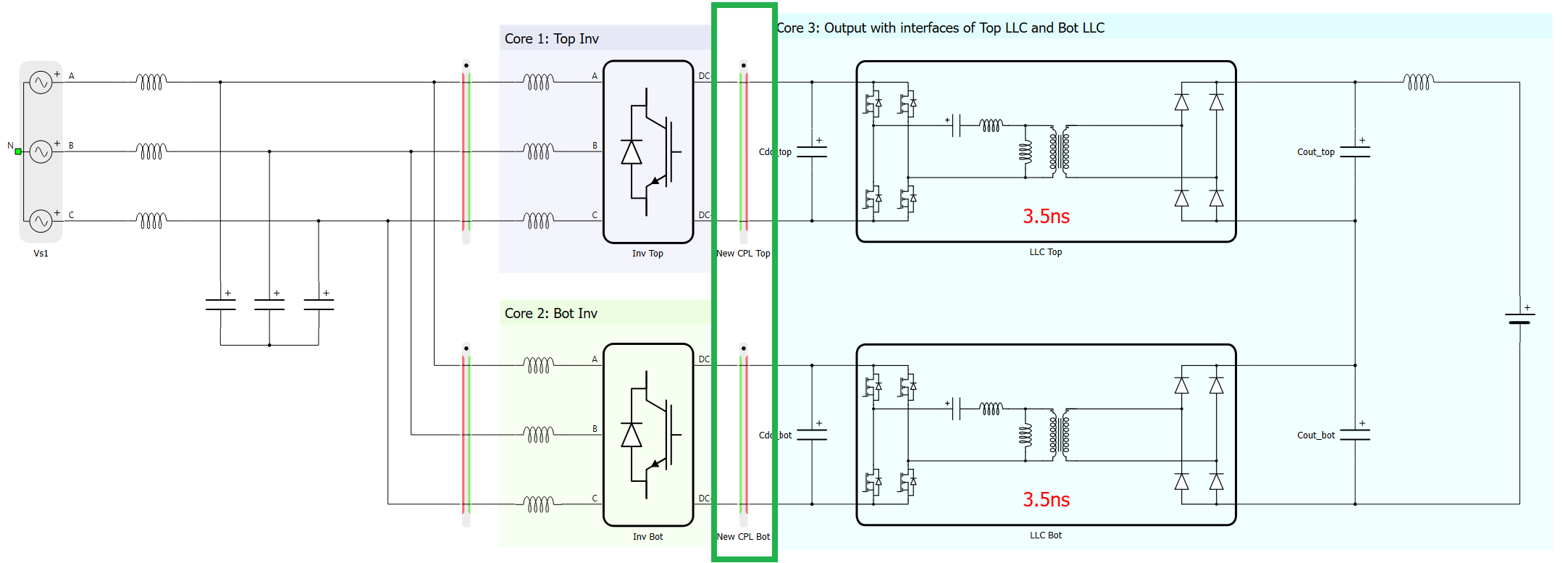
- Sides of the Electrical circuit interface are not decoupled, meaning that the input and the output side of the converter are placed into the same SPC, unlike with the old solver. This might lead to a situation in which the resources of said SPC are depleted, thus leading to unsuccessful compilation, or to a simulation with longer timestep than in the old model. Figure 3 shows how circuit partitioning of both power modules was handled by inherent decoupling that used to exist between the sides of the electrical circuit interface inside the solver. Since such decupling doesn't exist in the new solver, content of all three cores would end up in a single core, which would lead to unsuccessful compilation. In this case, the total converter weight would cause the compilation to fail. On a different model, matrix memory or any other computational resource might be depleted. A resolution for this particular model is shown in Figure 4. By adding two additional core coupling components (highlighted by the green rectangle), the model is repartitioned between the 3 cores, similar to how it was prior to the 2026.1 software update. Generally, it should be possible to place core coupling component(s) in a similar position in any model: inputs to DAB/resonant converters are dominantly acting as voltage sources (usually capacitor or a voltage source), meaning that a current side of an ideal transformer-based core coupling can be connected in parallel with the component that was at the DAB/resonant converter input.
- Total resource utilization of the Electrical circuit interface (both sides combined) is slightly increased. In a model in which two sides were explicitly put into the same core before the transition, time slot utilization of the said core will be increased by approximately 18 clock cycles of a HIL device (60 ns on HIL606, HIL506, and HIL404; 110 ns on HIL602+, and HIL604; 4.5 ns on HIL101). If the increase of the simulation timestep causes compilation to fail (time step value was specified to a fixed value), the specified step can be increased using steps of 50 ns until the compilation passes. If automatic determination of the timestep was used and the increased timestep is seen as relatively large, it is possible to specify the fixed step which can be only slightly larger than the previously used one. For example, if the automatically determined timestep increased from 250 ns to 500 ns (relatively large difference), 300 ns or 350 ns can be specified as a fixed step value. Compilation will pass and this minor timestep increase should not affect the simulation performance.