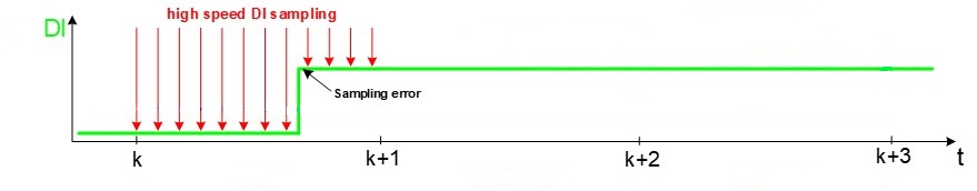
GDS oversampling
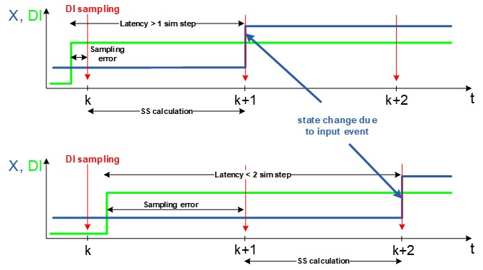
Definition and overview of GDS oversampling in real-time/VHIL simulation, and how it can be used in cases where it is needed to sample Digital inputs multiple times per simulation timestep.
GDS Oversampling in real-time/VHIL simulation
GDS (gate drive signals) is a digital input that is used to control the converter. In order to explain why GDS oversampling is needed and what is the the maximum frequency in which digital signals (GDSs) can be observed, let’s first define one term – the effective resolution. This resolution can be calculated by the following formula:
.
Since in most cases the fastest signals in a power electronics circuit are the Pulse-width modulation (PWM) gate drive signals, the effective resolution can be defined as the maximum resolution of the PWM that the HIL digital input sees for the given switching frequency. If, for example, there is a PWM signal with a resolution of 16 bits (which means 65000 different values of duty cycle), the effective resolution might be lower, depending on the PWM frequency and sampling time.
So far it is described how GDS oversampling is used to increase GDS sampling resolution. There are two different algorithms that rely on GDS oversampling in order to improve simulation results:
Please refer to the dedicated documentation for detailed information on these two algorithms. Global GDS oversampling can be enabled from Table 2, and it is enabled by default. Switch-level GDS oversampling is implemented at the component level, and it can be enabled in the component that supports it. It is important to note that when Switch-level GDS oversampling is enabled in a component, Global GDS oversampling will be ignored for that sub-circuit, even if it is enabled in settings. However, Global GDS oversampling will be executed for all other sub-circuits (SPCs).
GDS Oversampling frequency and minimum timestep
The GDS Oversampling resolution is defined by the IO timing of the device. More information is available in the IO Timing section of each HIL Simulator device's documentation. This means it can be as high as 6.25 ns for HIL402, 602+, and 604 devices, 4.5 ns for HIL101 devices, and 3.5 ns for HIL404, HIL506, and HIL606 devices.