Global GDS oversampling
Description of the global GDS oversampling feature, which greatly increases the frequency at which GDSs are sampled to avoid sampling errors. In cases where more than one GDS transition can happen during one simulation step, see Switch-level GDS oversampling instead.
Global GDS oversampling overview
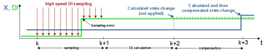
The motivation for GDS oversampling is explained in GDS oversampling document. So, here it is assumed that you are familiar with basic principle of the GDS oversampling. The main benefit of GDS oversampling is possibility to sample GDSs with much bigger frequency that the frequency of the simulation step. Global GDS Oversampling allows the HIL device to sample inputs multiple times during one simulation step while also memorizing the moment the change happened. By doing this, we can attenuate sampling errors, and reach far better simulation results. This works because with Global GDS Oversampling, information about the exact time when the GDS is changed is used to compensate the state output. Figure 1 shows an illustration of Global GDS oversampling on a simple example. The algorithm can be divided into three phases:
- Sampling of GDSs with high speed, and recording the moment when the change in the GDS happens.
- State space output is calculated with the wrong GDS input. Meanwhile, information about the time when the GDS changes is used to calculate the value of states that will be used for the compensation in the next simulation step. These values are not visible at the outputs.
- Third phase is the compensation of states. The temporary calculated state output from the previously simulated step and information about the time when the GDS is changed are used to calculate new state output. After calculation and compensation, the correct value of the state will be present at the output.
Drawbacks of Global GDS oversampling are:
- Additional computation load due to algorithm complexity and additional latency in the form of an additional time step dedicated for compensation.
- Only one GDS transition within each sub-circuit (SPC) can be handled during a single simulation step. In cases where more than one GDS transition can happen during one simulation step, see Switch-level GDS oversampling instead.
Global GDS oversampling can be enabled from Table 2, and it is enabled by default.
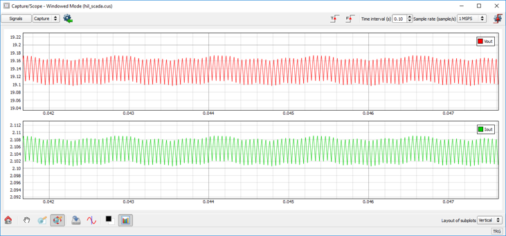
When using the Boost example model with a switching frequency of 20kHz and a PWM modulator block utilized in loop-back, we can see the difference between cases where Global GDS oversampling is used and when it is not. Figure 2 shows output voltage and current of a fixed PWM duty cycle in steady state operation with Global GDS Oversampling disabled. Fluctuations in both graphs are due to uncorrected sampling errors and are not expected in the real system. With a 1µS simulation step, the effective resolution is less than 6 bits. This means that simulator sees around 50 samples per PWM period, which results in imprecise duty cycle detection. Because of this, there are low frequency voltage and current fluctuations in the steady state with a fixed PWM duty cycle, which is something we do not expect to see in the real system.
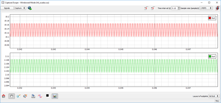
However, with Global GDS Oversampling enabled, the sampling period is much lower, which increases the effective resolution to around 13 or 12 bits. With this increased number of samples per PWM period and with an algorithm that uses the exact time when GDS is changed to compensate state output, we have much more accurate results which can be seen in Figure 3, where unexpected fluctuations do not exist.
GDS Oversampling frequency and minimum timestep
The GDS Oversampling resolution is defined by the IO timing of the device. More information is available in the IO Timing section of each HIL Simulator device's documentation. This means it can be as high as 6.25 ns for HIL402, 602+, and 604 devices, 4.5 ns for HIL101 devices, and 3.5 ns for HIL404, HIL506, and HIL606 devices.