SFP with Modular Multi-level Converter (MMC)
Demonstration of the capabilities of Aurora Small Form-factor Pluggable (SFP) simulation link to establish communication between a HIL device and a controller.
Introduction
SFP Simulation Link is a bidirectional, open protocol interface that allows high bandwidth, low latency data exchange with the outside world. This link allows you to directly interact with another FPGA microprocessor over SFP Simulation Link. It also gives you more flexibility with your analog and digital IO slots, by allowing your controller to send IO signals to the HIL over SFP instead.
This application note demonstrates the capabilities of establishing Aurora Small Form-factor Pluggable (SFP) simulation link communication between a HIL device and a controller. It is supported by generation 4 HIL devices (HIL101, HIL404, HIL506 and HIL606). The upper SFP connector is used for communication when SFP link components are present in the model, leaving the bottom SFP connector available for device paralleling, as shown on the left in Figure 1. The right portion of the figure shows how you could connect an SFP link to a real controller, which is not covered in this example.
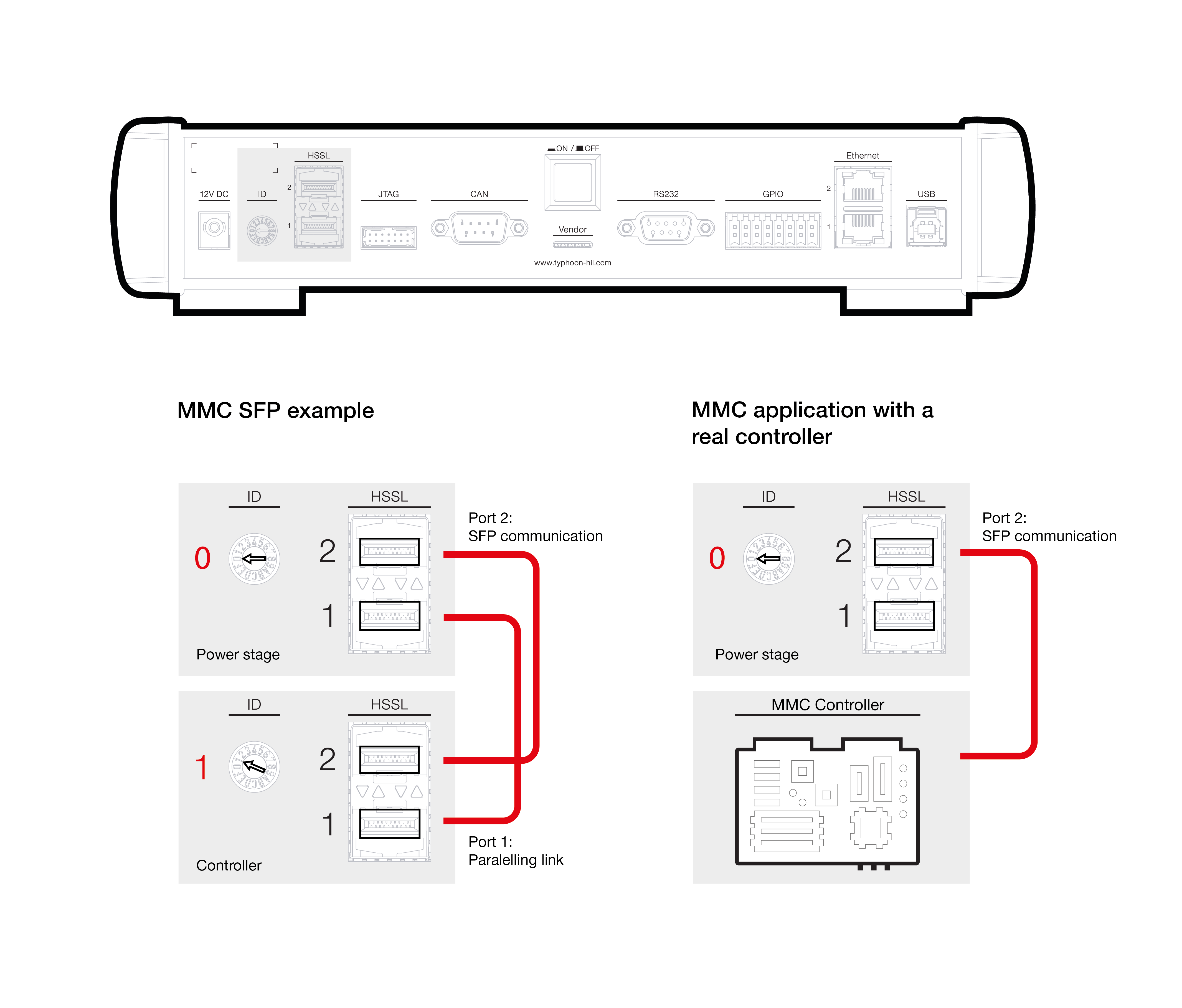
In this example, we are using a multi-HIL setup consisting of two HIL devices that support SFP. The HILs are connected using two SFP Fiber Cables. The HIL device with ID0 acts as the power stage, while the HIL device with ID1 behaves as the controller side. Additional information about paralleling HIL devices is available in the HIL Paralleling Guide or in our video knowledgebase (Video: 3.3.3 Introduction to device partitioning).
You can find more information about the MMC structure and topology here: Introduction
Model description
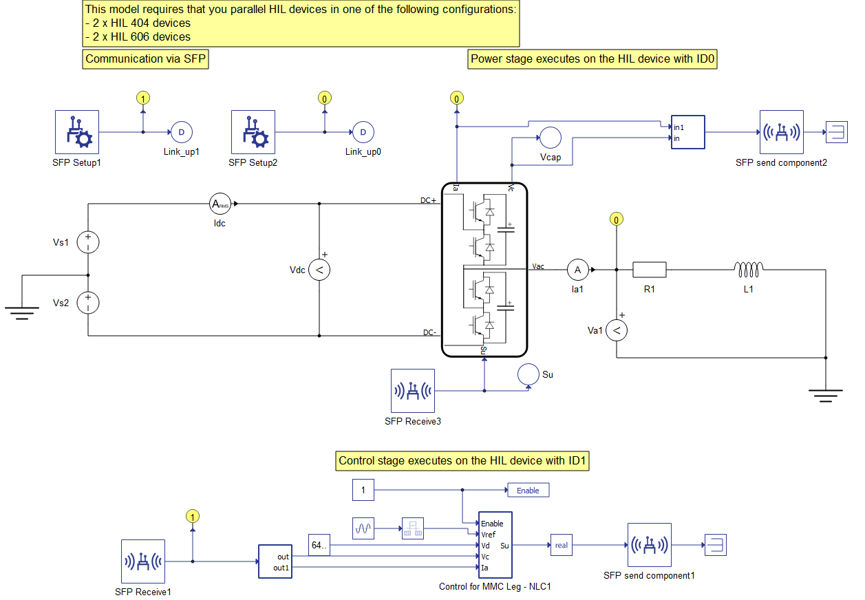
The model consists of a DC link, a MMC Leg - Switching Function with Nearest Level Control (NLC), and a constant load, and two pairs of SFP send and SFP receive blocks. Also, this model consists of two SFP setup blocks, one for each HIL device. The SFP send component in HIL device ID0 sends signals with the voltages of the sub-modules and currents in the upper and lower legs to the controller. The controller in HIL device ID1 receives the signals and provides them as inputs to the control algorithm. The control algorithm then sends the gate signals to the sub-modules in the single phase MMC leg.
Simulation
This application comes with a pre-built SCADA panel. The panel offers most essential user interface elements (widgets) to monitor and interact with the simulation in runtime. You can customize it freely to fit your needs.
The SCADA panel made for this MMC converter model allows you to have a broad insight into the operation of this converter through its various widgets and scopes. In the two groups on the left side of the SCADA, you can observe the up-capacitor voltage and down capacitor voltage of a few sub-modules. In the Trace graphs at the bottom left, you can see the up-capacitor voltage and down capacitor voltage of a few sub-modules.
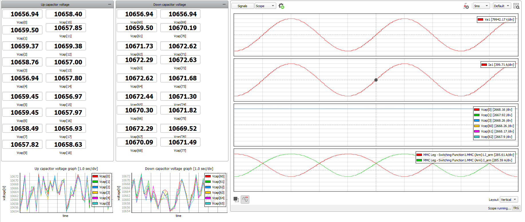
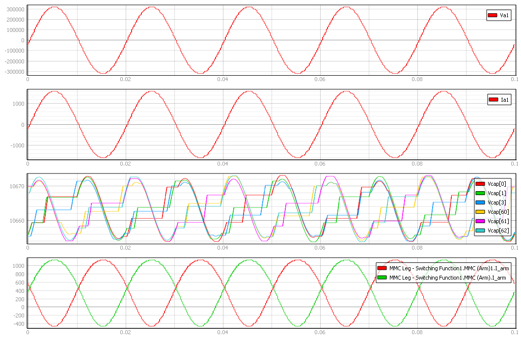
In Capture, you can see the current, voltages, voltages on sub-module capacitors, and up and down arm currents. In the third viewport, capacitor voltages are shown, which demonstrates how the controller balances voltages on the capacitors. In the last viewport the upper arm current and lower arm current are shown.
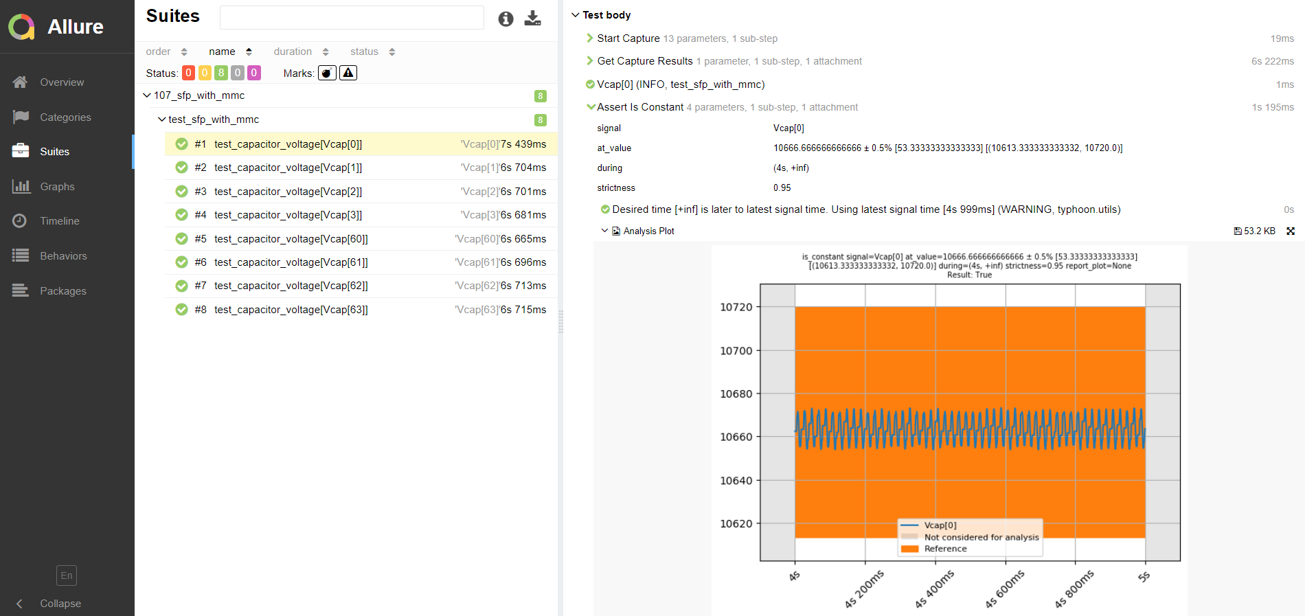
Test Automation
The provided test automation script validates if the voltage on each of the 8 capacitors in the submodule are within an expected tolerance. The test captures the first five seconds of the simulation. When the voltages of the sub-module capacitors are in a steady state, the test measures and compares these values with the expected value , which is 10.66 kV in this case. The tolerance is 0.5%, which is approximately 50 V.
Example requirements
Table 1 provides detailed information about the file locations and hardware requirements for running the model in real-time, followed by the HIL device resource utilization when running the model using this minimal hardware configuration. This information is provided to help you with running and customizing the model as you see fit.
| Files | |
|---|---|
| Typhoon HIL files |
examples\models\communication protocols\sfp with mmc\ sfp with mmc.tse sfp with mmc.cus examples\tests\107_sfp_with_mmc\ test_sfp_with_mmc.py |
| Minimum hardware requirements | |
| No. of HIL devices | 2 |
| HIL device model | HIL101 |
| HILCore configuration | Base 1 |
| HIL device resource utilization | |
| No. of processing cores | 1 per device |
| Max. matrix memory utilization | HIL1 0.02% (core0) HIL0 0.24% (core0) |
| Max. time slot utilization | HIL1 43.64% (core0) HIL0 60.0% (core0) |
| Simulation step, electrical | 250 ns |
| Execution rate, signal processing | Multirate (50 µs, 250 µs) |
Authors
[1] Simisa Simic