Generic battery

Introduction

The use of microgrids has been steadily increasing over the last few years, and so has been the need to model and test their control systems. In short, the microgrid field is currently on the rise, accompanied by a growing need for more efficient microgrid components.

This application note describes the main characteristics of a battery inverter and presents a use case typical for generic components.

Model description

The model consists of a Battery EES (Generic) connected to the Grid with corresponding UI components and a passive load that can be connected or disconnected.

Figure 1: Battery inverter connected on the grid

Figure 2: Battery ESS (generic) properties

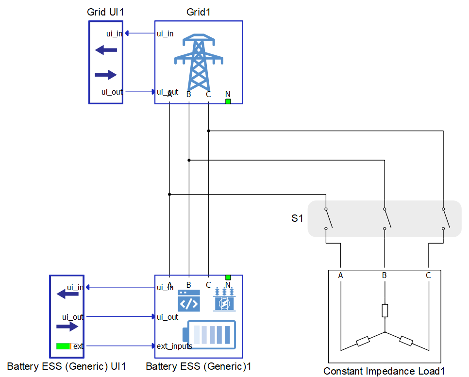
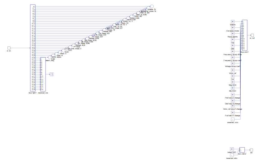
Unlike common microgrid components where you need to define all inputs and outputs, generic components have a user interface where all the inputs and outputs necessary for the operation of the General Battery are already defined. Because this block is unlocked, there is also a possibility for adding additional, user-specific functionalities and improvements such as communication interfaces or optimization logic. In addition to the usual inputs and outputs set by the power management system, there are also external inputs related to system specific factors. In this case, the external input is the initial State Of Charge (SOC).

Figure 3: Second-level UI of the Battery ESS (generic) component

Simulation

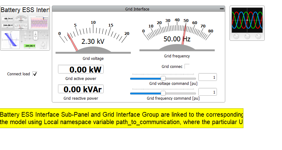
This application comes with a pre-built SCADA panel shown in Figure 4. It offers the most essential user interface elements (widgets) to monitor and interact with the simulation at runtime, allowing you to further customize it according to your needs.

The inverter can operate in the following three operation modes:

• grid following
• droop
• isochronous

  Figure 4: SCADA_panel

  

In addition to the three operational modes, the inverter also has four operational states: 

• Disabled – the state when the inverter is turned off and the main circuit breaker is open. 
• Starting up - the state of the converter between the moment of enabling signal activation and the moment when the converter starts operating, e.g. the synchronization time. 
• Running state – the state when the inverter is operating. 
• Fault state – the state when a fault is detected. If the inverter is in the error state, in order to start the plant again, it is necessary to reset the alarm. 

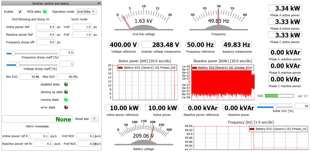
Figure 5 shows the part with the inverter control where you can read the state of the inverter as well as get information if protection is active. Here you can also read the measurements of active and reactive power, voltage and frequency measurements, and SOC. Figure 5 also represents the case when the inverters operates in the grid-following mode, in which you can change active and reactive power.

Figure 5: Battery ESS (generic) Interface in the grid-following mode

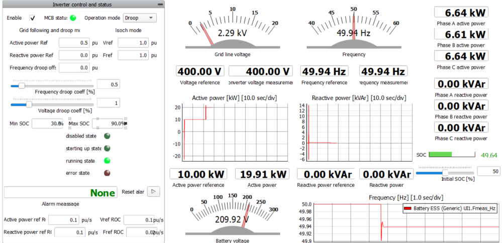
As mentioned above, one of the characteristics of generic components is that they can operate in two grid-forming modes: droop mode and isochronous mode. When droop mode is chosen, it means that you can set references for active and reactive power. Unlike in grid-following mode, the inverter can operate when disconnected from the grid, with its operation is defined by its droop characteristic. Figure 6 shows the case when the inverter operates in droop mode parallel with the grid. After approximately 2 seconds, the grid is disconnected and the battery inverter forms the grid. The frequency is 49.88 Hz instead of 50 Hz because of the defined droop characteristic. The frequency droop characteristic is defined by the coefficient and offset values.

Figure 6: Battery ESS (generic) Interface in the droop mode

In isochronous mode, voltage and frequency are set directly, as in Figure 7.

Figure 7: Battery ESS (generic) Interface in the isochronous mode

Fault detection is something that separates generic components from switching and average ones. Generic components can detect five types of faults:

• Over-current protection - when some of the input phase currents are 1.5 times over the maximum allowed instantaneous current
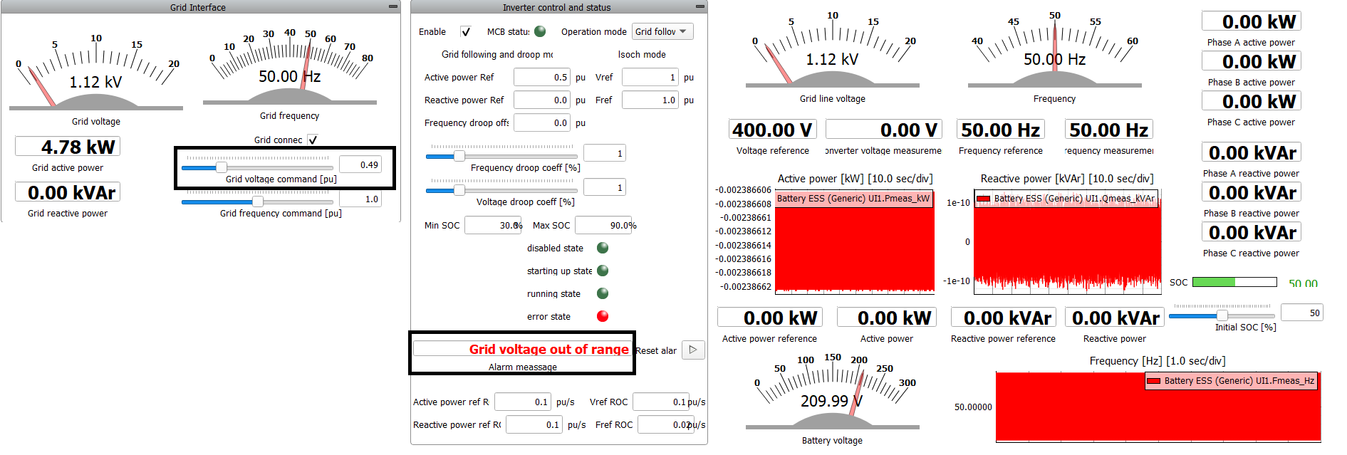
• Grid voltage out of range - when the grid voltage is outside the specified relative range [0.5, 1.5] pu. This protection is active in grid-following mode
• Grid frequency out of range - when the grid frequency is outside the specific relative range [0.5, 1.5] pu. This protection is active in grid-following mode
• Over-power protection - when the measured apparent power is more than 1.2 times greater than the maximum allowed apparent power. This protection is active in grid-forming mode.
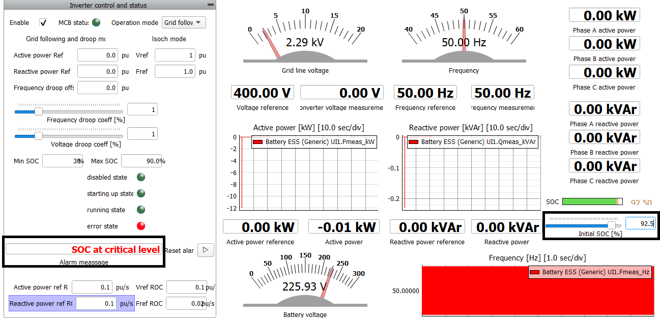
• SOC at critical level - If the SOC is higher than Max SOC + 2% or lower than Min SOC - 2% this fault will be generated.

Figure 8: Grid-voltage-out-of-range protection is activated

Figure 9: SOC-at-critical-level protection is activated