abc_to_symmetrical_components

typhoon.test.transformations.abc_to_symmetrical_components(signals: DataFrame, method: str = 'Fortescue', output: str = 'Complex', mag_in_rms: bool = True, angle_in_degrees: bool = True)

Implements the Symmetrical transformation, also known as Fortescue transform.

The Symmetrical transformation splits the unbalanced 3-phases signals into three balanced signal with the zero, positive and negative sequences.

This function allows input of sine or complex sine values. For sine signals (not complex values), such as the three-phase generated by typhoon.test.signals.pandas_3ph_sine(), the Hilbert Transform will be used to split the real and imaginary component of the sine function. For complex signals, the Hilbert transform is not applied, and only the symmetrical components transform is performed.

The sequences (zero, positive, and negative) from the symmetrical components can be represented by complex or phasor values.

Parameters:

• signals (pandas.DataFrame) – Signals with three columns, one for every signal of the three-phase abc input. Signals can be complex or sinusoidal.

• method (string) – Selects the transformation method. Allowed values are 'Fortescue', or 'Power invariant'; other values will raise an exception. Default is method='Fortescue'

• output (string) –

  Selects the output type. Allowed values are 'Complex', or 'Phasor'; other values will raise an exception. If 'Complex' is selected this function will return:

  • A pandas.DataFrame with three columns, one for each output signal.

  The labels to select the columns are 'zero', 'positive' and 'negative', respectively.

  If 'Phasor' is selected this function will return:

  • A pandas.DataFrame with six columns, one for each symmetrical component (magnitude and phase).

  The labels to select the columns are, respectively:

  • "zero_mag": Magnitude of Zero Component

  • "zero_phase": Phase of Zero Component

  • "pos_mag": Magnitude of Positive Component

  • "pos_phase": Phase of Positive Component

  • "neg_mag" : Magnitude of Negative Component

  • "neg_phase": Phase of Negative Component

  Default is output='Complex'.

• mag_in_rms (bool) – If this option is True and output='Phasor' the magnitude of the symmetrical components in the pandas.DataFrame will be return with values in RMS. If this option is False, amplitude values will be returned. Default is mag_in_rms=True.

• angle_in_degrees (bool) – If this option is True and output='Phasor' the angle of the symmetrical components in the pandas.DataFrame will be return with values in degrees. If this option is False, values will be returned in radians. Default is angle_in_degrees=True.

Returns:

DataFrame containing the symmetrical components, the columns size and label depends on the chosen 'output'.

Return type:

pandas.DataFrame

Examples

In this example the instantaneous mode of the function is used. The three-phase sines are used as signals. These are decomposed into complex values, using Hilbert Transform, which are then used to calculate the symmetrical components.

>>> from typhoon.test.transformations import abc_to_symmetrical_components
>>> from typhoon.test.signals import pandas_3ph_sine
>>>
>>> amplitude = 311
>>> frequency = 50
>>> duration = 1
>>> Ts = 1e-4
>>>
>>> signals = pandas_3ph_sine(amplitude, frequency, duration, Ts)
>>>
>>> zpn_fortescue = abc_to_symmetrical_components(signals)  # Implicit method = "Fortescue"
>>> zpn_power_inv = abc_to_symmetrical_components(signals, method="Power invariant")

The zpn_fortescue and zpn_power_inv will both be pandas.DataFrame with three columns of complex:

• "zero" with the balanced zero components,

• "positive" with the balanced positive components,

• "negative" with the balanced negative components

The zpn_fortescue components are shown in the plot: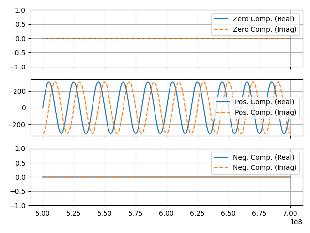

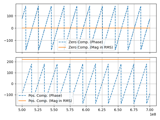
And to get the symmetrical components as magnitude and phase:

>>> zpn_fortescue_phasor = abc_to_symmetrical_components(
>>>     signals, output="Phasor"
>>> )  # Implicit method = "Fortescue"

The zpn_fortescue_phasor zero and positive components are shown in the plot:

See also

typhoon.test.transformations.abc_to_alphabetagamma, typhoon.test.transformations.abc_to_dq0, typhoon.test.transformations.symmetrical_components_to_abc