Six Phase Permanent Magnet Synchronous Machine (Double Stator)
Description of the Six Phase Permanent Magnet Synchronous Machine (Double Stator) component in Schematic Editor.
| component | component dialog window | component parameters |
|---|---|---|
 |
 |
|
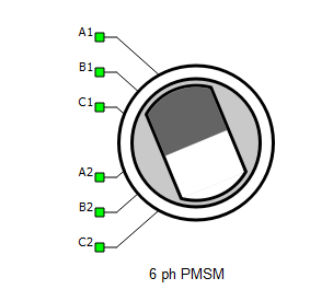
A1, B1, and C1 are the stator winding 1 terminals. A2, B2, and C2 are the stator winding 2 terminals. Both of the windings use the current source interface.
Electrical sub-system model
The electrical part of the machine is represented by the following system of equations, modeled in the rotating dq reference frame. The dq reference frame is attached to the rotor.
If the linear model is chosen on the component's mask, the d-axis is aligned with the rotor magnets and q-axis permanent magnet flux is not considered ( ). The q-axis permanent magnet flux is taken into consideration only in the nonlinear machine model.
If the saturation effects are considered, the equations have the same form, but in that case, fluxes and inductances are functions of stator currents:
In the equations listed above, ids current represents a sum of d-axis currents of both three phase machine stator windings:
and iqs current represents a sum of q-axis currents of both three phase machine stator windings:
| symbol | description |
|---|---|
| ψds1 | Direct axis component of stator winding 1 flux [Wb] |
| ψqs1 | Quadrature axis component of stator winding 1 flux [Wb] |
| ψds2 | Direct axis component of stator winding 2 flux [Wb] |
| ψqs2 | Quadrature axis component of stator winding 2 flux [Wb] |
| ψPMd | Direct axis component of flux amplitude established in stator phases by rotor permanent magnets [Wb] |
| ψPMq | Quadrature axis component of flux amplitude established in stator phases by rotor permanent magnets [Wb] |
| ids1 | Direct axis component of stator winding 1 current [A] |
| iqs1 | Quadrature axis component of stator winding 1 current [A] |
| ids2 | Direct axis component of stator winding 2 current [A] |
| iqs2 | Quadrature axis component of stator winding 2 current [A] |
| vds1 | Direct axis component of stator winding 1 voltage [V] |
| vqs1 | Quadrature axis component of stator winding 1 voltage [V] |
| vds2 | Direct axis component of stator winding 2 voltage [V] |
| vqs2 | Quadrature axis component of stator winding 2 voltage [V] |
| Rs | Stator phase resistance [Ω] |
| Ld | Direct axis inductance [H] |
| Lq | Quadrature axis inductance [H] |
| Md | Direct axis coupling inductance of stator windings [H] |
| Mq | Quadrature axis coupling inductance of stator windings [H] |
| ωr | Rotor electrical speed [rad/s] ( ) |
| p | Machine number of pole pairs |
| Te | Machine developed electromagnetic torque [Nm] |
Mechanical sub-system model
Motion equation:
| symbol | description |
|---|---|
| ωm | Rotor mechanical speed [rad/s] |
| Jm | Combined rotor and load moment of inertia [kgm2] |
| Te | Machine developed electromagnetic torque [Nm] |
| Tl | Shaft mechanical load torque [Nm] |
| b | Machine viscous friction coefficient [Nms] |
| θm | Rotor mechanical angle [rad] |
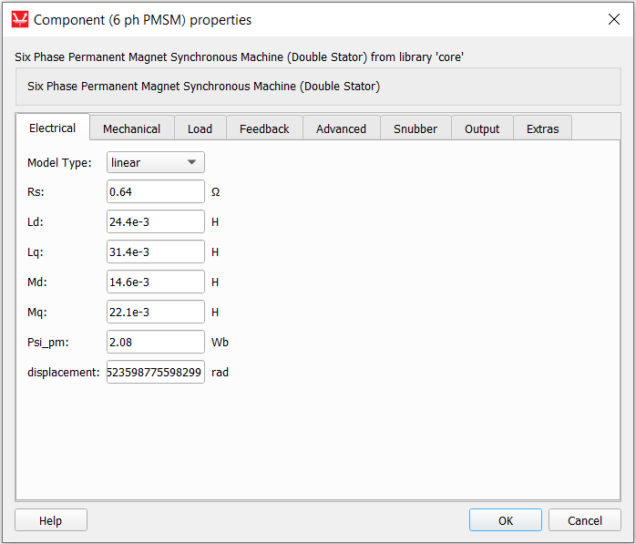
Electrical
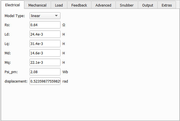
- linear
- nonlinear
- absolute inductance vs current
| symbol | description |
|---|---|
| Rs | Stator phase resistance [Ω] |
| Ld | Direct axis inductance [H] |
| Lq | Quadrature axis inductance [H] |
| Md | Direct axis coupling inductance of stator windings [H] |
| Mq | Quadrature axis coupling inductance of stator windings [H] |
| Psi_pm | Flux amplitude established in stator phases by rotor permanent magnets [Wb] |
| id vector | List of stator current direct axis component values [A] |
| iq vector | List of stator current quadrature axis component values [A] |
| Ld table | Table of stator self inductance direct axis component values [H] |
| Lq table | Table of stator self inductance quadrature axis component values [H] |
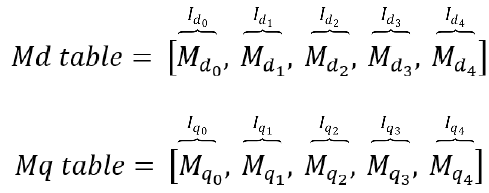
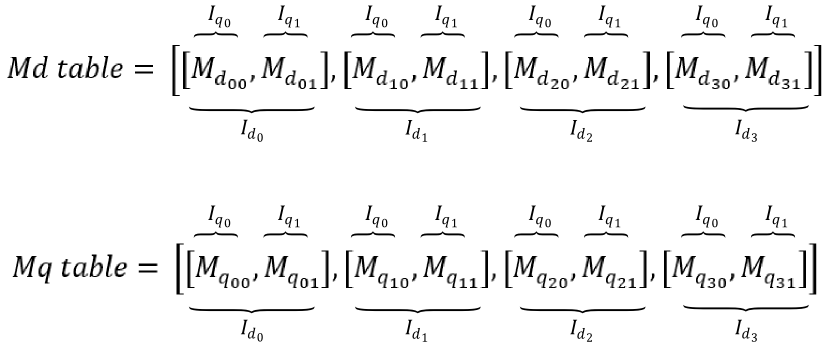
| Md table | Table of stator windings coupling inductance direct axis component values [H] |
| Mq table | Table of stator windings coupling inductance quadrature axis component values [H] |
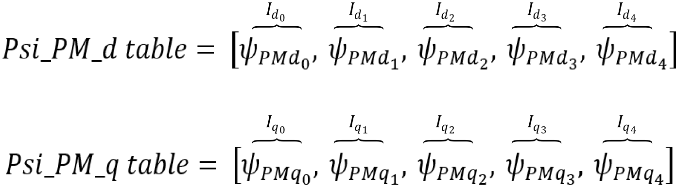
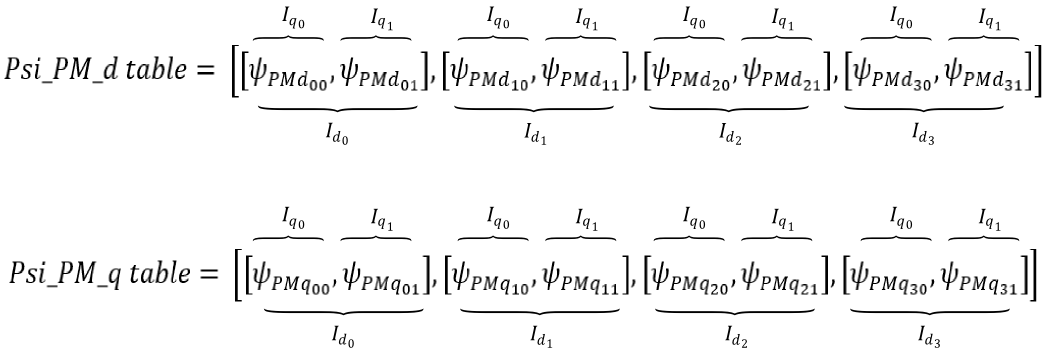
| Psi_pm_d table | Table of stator permanent magnet flux direct axis component values [Wb] |
| Psi_pm_q table | Table of stator permanent magnet flux quadrature axis component values [Wb] |
| displacement | Electrical angle displacement between the stator windings, measured from winding 2 to winding 1 [rad] |
The Six Phase Permanent Magnet Synchronous Machine model can include magnetic saturation effects. In that case, self and coupling inductances, as well as the permanent magnet fluxes are defined as functions of stator currents and . These functions are represented in the form of lookup tables. The lookup tables use linear interpolation and linear extrapolation.
- absolute inductances vs stator currents
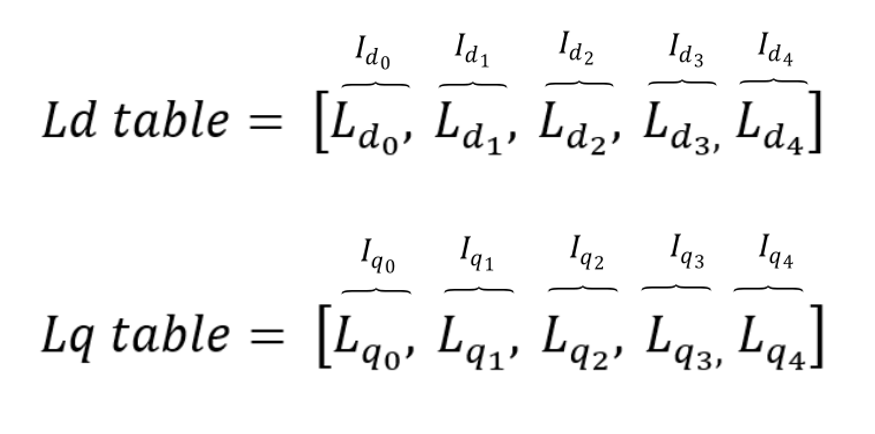
id_vector = [-40.0, -20.0, 0.0, 20.0, 40.0]
iq_vector = [-40.0, -20.0, 0.0, 20.0, 40.0]
Ld_table = [0.00186383, 0.00325188, 0.00399657, 0.00136793, 0.000562082]
Lq_table = [0.00321572, 0.00538029, 0.00779154, 0.00535, 0.00319568]
Md_table = [0.0013978724999999998, 0.00243891, 0.0029974274999999997, 0.0010259475, 0.0004215615]
Mq_table = [0.00241179, 0.0040352175, 0.005843655, 0.0040125, 0.00239676]
Psi_PM_d_table = [-0.0492472, -0.0433668, -0.0425532, -0.0433464, -0.0484104]
Psi_PM_q_table = [-0.1330824, -0.0838922, 0.0, 0.0838828, 0.133098]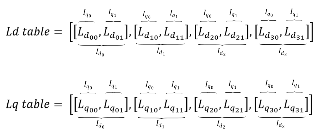
id_vector = [-40.0, -20.0, 0.0, 20.0, 40.0]
iq_vector = [-40.0, -20.0, 0.0, 20.0, 40.0]

Ld_table = [[0.00203118, 0.00188417, 0.00186383, 0.00188366, 0.00201026],
            [0.00217976, 0.00297238, 0.00325188, 0.0029855, 0.00223459],
            [0.00226518, 0.00283656, 0.00399657, 0.00280727, 0.00218666],
            [0.0016353, 0.00171137, 0.00136793, 0.00178913, 0.00164534],
            [0.00121342, 0.00096362, 0.000562082, 0.000967825, 0.00123179]]

Lq_table = [[0.00332706, 0.00419461, 0.0049565, 0.00419414, 0.00332745],
            [0.00328404, 0.00520506, 0.00635444, 0.00520574, 0.00320567],
            [0.00321572, 0.00538029, 0.00779154, 0.00535, 0.00319568],
            [0.00293984, 0.00421955, 0.00547829, 0.00419697, 0.00290709],
            [0.00273112, 0.00294274, 0.00323358, 0.00292902, 0.00271144]]

Md_table = [[0.00152338, 0.00141313, 0.00139787, 0.00141274, 0.00150769],
            [0.00163482, 0.00222929, 0.00243891, 0.00223912, 0.00167594],
            [0.00169888, 0.00212742, 0.00299743, 0.00210545, 0.00163999],
            [0.00122647, 0.00128353, 0.00102595, 0.00134185, 0.001234],
            [0.00091007, 0.00072271, 0.00042156, 0.00072587, 0.00092384]]

Mq_table = [[0.0024953, 0.00314596, 0.00371738, 0.00314561, 0.00249559],
            [0.00246303, 0.00390379, 0.00476583, 0.00390431, 0.00240425],
            [0.00241179, 0.00403522, 0.00584365, 0.0040125, 0.00239676],
            [0.00220488, 0.00316466, 0.00410872, 0.00314773, 0.00218032],
            [0.00204834, 0.00220706, 0.00242518, 0.00219676, 0.00203358]]

Psi_PM_d_table = [[-0.0492472, -0.0433668, -0.0425532, -0.0433464, -0.0484104],
                  [-0.0115952, -0.0274476, -0.0330376, -0.02771, -0.0126918],
                  [0.032, 0.032, 0.032, 0.032, 0.032],
                  [0.064706, 0.0662274, 0.0593586, 0.0677826, 0.0649068],
                  [0.0805368, 0.0705448, 0.05448328, 0.070713, 0.0812716]]

Psi_PM_q_table = [[-0.1330824, -0.0838922, 0.0, 0.0838828, 0.133098],
                  [-0.1313616, -0.1041012, 0.0, 0.1041148, 0.1282268],
                  [-0.1286288, -0.1076058, 0.0, 0.107, 0.1278272],
                  [-0.1175936, -0.084391, 0.0, 0.0839394, 0.1162836],
[-0.1092448, -0.0588548, 0.0, 0.0585804, 0.1084576]]Mechanical
| symbol | description |
|---|---|
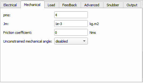
| pms | Machine number of pole pairs |
| Jm | Combined rotor and load moment of inertia [kgm2] |
| Friction coefficient | Machine viscous friction coefficient [Nms] |
| Unconstrained mechanical angle | Limiting mechanical angle between 0 and 2π |
Load
| symbol | description |
|---|---|
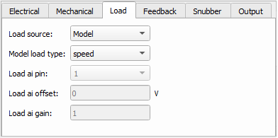
| Load source | Load can be set from SCADA/external or from model (in model case, one signal processing input will appear) |
| External/Model load type | External/Model load type: torque or speed |
| Load ai pin | HIL analog input address for external torque command |
| Load ai offset | Assigned offset value to the input signal representing external torque command |
| Load ai gain | Assigned gain value to the input signal representing external torque command |
External load enables you to use an analog input signal from a HIL analog channel with the load_ai_pin address as an external torque/speed load, and to assign offset (V) and gain (Nm/V) to the input signal, according to the formula:
Feedback
| symbol | description |
|---|---|
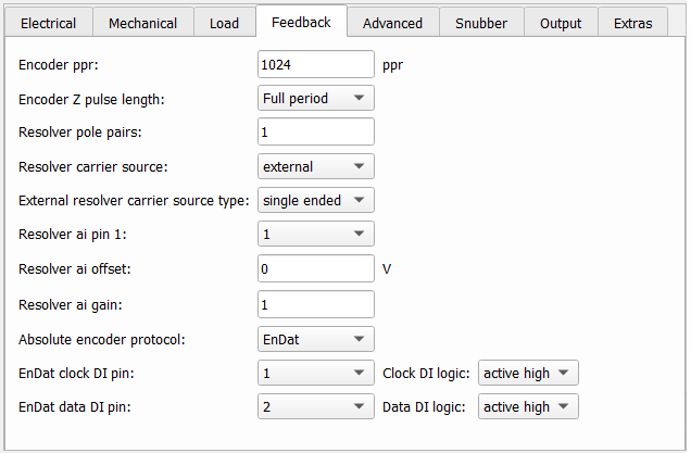
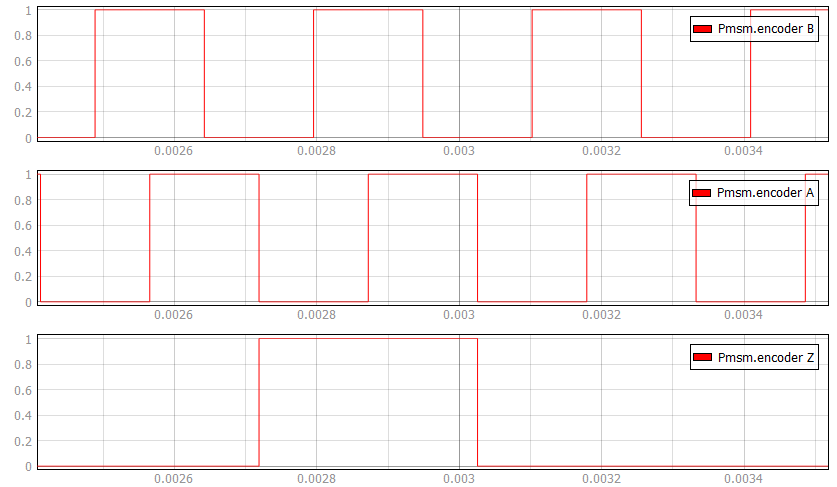
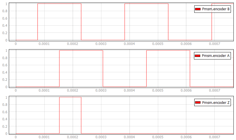
| Encoder ppr | Incremental encoder number of pulses per revolution |
| Encoder Z pulse length | Z digital signal pulse length in periods. Can be Quarter length or Full period (default) |
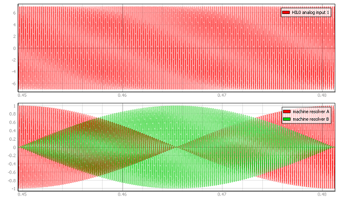
| Resolver pole pairs | Resolver number of pole pairs |
| Resolver carrier source | Resolver carrier signal source selection (internal or external) |
| External resolver carrier source type | External resolver carrier signal source type selection (single ended or differential); available only if the Resolver carrier source property is set to external |
| Resolver carrier frequency | Resolver carrier signal frequency (internal carrier) [Hz] |
| Resolver ai pin 1 | Resolver carrier input channel 1 address (external carrier) |
| Resolver ai pin 2 | Resolver carrier input channel 2 address (external carrier); available only if the External resolver carrier source type property is set to differential |
| Resolver ai offset | Resolver carrier input channel offset (external carrier) |
| Resolver ai gain | Resolver carrier input channel gain (external carrier) |
| Absolute encoder protocol | Standardized protocol providing the absolute machine encoder position |
If an external resolver carrier source is selected, the source signal type can be set as either single ended or differential. The single ended external resolver carrier source type enables use of an analog input signal from the HIL analog channel with the res_ai_pin_1 address as the external carrier source. Additionally, offset (V) and gain (V/V) values can be assigned to the input signal, according to the formula:
The differential external resolver carrier source type enables use of two analog input signals from the HIL analog channels with the res_ai_pin_1 and the res_ai_pin_2 addresses. Analog signals from these HIL analog inputs are subtracted, and the resulting signal is used as the external differential carrier source. Additionally, offset (V) and gain (V/V) values can be assigned to the input signal (similarly to the single ended case), according to the formula:
The following expression must hold in order to properly generate the encoder signals:
| symbol | description |
|---|---|
| enc_ppr | Encoder number of pulses per revolution |
| fm | Rotor mechanical frequency [Hz] |
| Ts | Simulation time step [s] |
Advanced
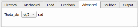
| symbol | description |
|---|---|
| Theta_ab | Position of the stationary αβ reference frame, in respect to the stator phase a axis [rad] |
The machine model output variables (currents, voltages and fluxes) can be observed from a stationary reference frame. There are two widely used approaches in electrical machine modeling: in the first, the alpha axis of the stationary reference frame lags by 90 degrees in regard to the stator phase a axis (used by default, and indicated in a) Figure 6. In the second one, the alpha axis is aligned with the stator phase a axis (indicated in b) Figure 6. The user can select between these two situations.
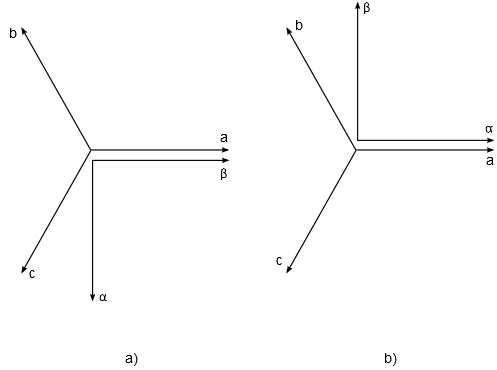
It is important to know the value of Theta_ab when the rotor position feedback is necessary. As an example, if a model uses the mechanical angle as a feedback signal and feeds it to one of the abc to dq, alpha beta to dq, dq to abc, or dq to alpha beta transformation blocks, the same transformation angle offset value should be used in both components to ensure the expected simulation results.
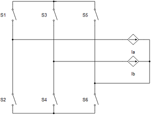
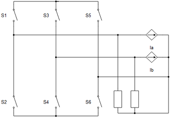
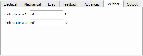
Snubber
All machines with current source based circuit interfaces have the Snubber tab in the properties window where the value of snubber resistance can be set. Snubbers are necessary in the cases when an inverter or a contactor is directly connected to the machine terminals. This value can be set to infinite (inf), but it is not recommended when a machine is directly connected to the inverter since there will be a current source directly connected to an open switch. In this case, one of each switch pairs S1 and S2, S3 and S4, and S5 and S6 will be forced closed by the circuit solver in order to avoid the topological conflicts. On the other hand, with finite snubber values, there's always a path for the currents Ia and Ib, so all inverter switches can be open in this case. Circuit representations of this circuit without and with snubber resistors are shown in Figure 4 and Figure 5 respectively. Snubbers are connected across the current sources.
| symbol | description |
|---|---|
| Rsnb stator w1 | Stator winding 1 snubber resistance value [Ω] |
| Rsnb stator w2 | Stator winding 2 snubber resistance value [Ω] |
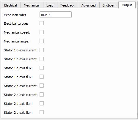
Output
This block tab enables a single, vectorized signal output from the machine. The output vector contains selected machine mechanical and/or electrical variables in the same order as listed in this tab.
| symbol | description |
|---|---|
| Execution rate | Signal processing output execution rate [s] |
| Electrical torque | Machine electrical torque [Nm] |
| Mechanical speed | Machine mechanical angular speed [rad/s] |
| Mechanical angle | Machine mechanical angle [rad] |
| Stator 1 d-axis current | Direct axis component of the stator 1 current [A] |
| Stator 1 q-axis current | Quadrature axis component of the stator 1 current [A] |
| Stator 1 d-axis flux | Direct axis component of the stator 1 flux [Wb] |
| Stator 1 q-axis flux | Quadrature axis component of the stator 1 flux [Wb] |
| Stator 2 d-axis current | Direct axis component of the stator 2 current [A] |
| Stator 2 q-axis current | Quadrature axis component of the stator 2 current [A] |
| Stator 2 d-axis flux | Direct axis component of the stator 2 flux [Wb] |
| Stator 2 q-axis flux | Quadrature axis component of the stator 2 flux [Wb] |